Problem
Because of physical constraints, economical constraints, time constraints or other constraints, it is usually impractical to gather information from every unit within a population to determine the characteristics of the population. For decision making, data analysts want to use inferential statistics to estimate the population parameters from sample statistics. For instance, Adventure Works Cycles [1], a fictitious company, has 18,484 registered customers. Knowledge of the average income of these customers and the proportion of bike buyers in all customers help to make marketing decisions. How do data analysts use inferential statistics to draw conclusions about population parameters by using sample statistics?
Solution
The Microsoft sample database AdventureWorksDW2017[1] contains a list of 18,484 customers. We can access the list through the view “vTargetMail”. Even though the view includes the columns “YearlyIncome” and “BikeBuyer”, for demonstration purposes, we assume that we do not have data in these two columns. Thus, we cannot compute the average value of customer yearly income or count the number of bike buyers directly from the database table. We also have an assumption that the population standard deviation of customer yearly income is 32,285. When we have a considerable amount of historical data, we can have this kind of assumption [2]. We use an unbiased estimator when the population standard deviation is unknown.
We randomly selected 35 participants from the customer list who reported their yearly incomes and told whether they owned a bike. With the sample of 35 observations, we constructed confidence intervals that contain the true values of the population mean and proportion, respectively. This tip shows a step-by-step solution to use sample statistics to estimate population parameters.
This tip is organized as follows. In Section 1, we explore concepts of statistical parameter estimation with some practice examples. Section 2 introduces the construction of large-sample confidence interval for the population mean. We construct a large-sample confidence interval for the population proportion in Section 3. Next, in Section 4, we briefly introduce parameter estimation for a small sample where the sample size is less than or equal to 30.
I tested all the source codes used in this tip with SQL Server Management Studio V18.3.1, Microsoft Visual Studio Community 2017 and Microsoft R Client 3.4.3 on Windows 10 Home 10.0 <X64>. The DBMS is Microsoft SQL Server 2017 Enterprise Edition (64-bit).
1 – Statistical Parameter Estimation
There are two branches of statistics: descriptive statistics and inferential statistics [3]. Descriptive statistics summarizes and presents data in a meaningful way. Inferential statistics provides methods that allow us to estimate the parameters of a population from which we drew the samples.
In this section, we illustrate some concepts involved in parameter estimation. Another important type of inferences is the testing of statistical hypotheses, which is beyond the scope of this tip. I assume you have had some previous experience with probability, random variables and their distributions, and sampling.
1.1 Unbiased Estimator
When a sample statistic is used to estimate a population parameter, we call this statistic an estimator of the parameter. For example, when we use a sample mean to estimate a population mean, the sample mean is an estimator of the population mean. If the expected value of the sampling distribution of a statistic is equal to the value of the population parameter being estimated, we consider this statistic to be an unbiased estimator of the parameter. For instance, the mean of the sampling distribution of the means is equal to the population mean, therefore, the sample mean is an unbiased estimator of the population mean.
To be an unbiased estimator, a sample statistic should have two desired properties: (1) the sampling distribution of the statistic centers at the parameter, and (2) the statistic has a small standard error [4]. Table 1 shows a list of unbiased estimators. We use a sample mean to estimate the population mean, use a sample proportion to estimate the population proportion, and use a sample standard deviation to estimate the population standard deviation.

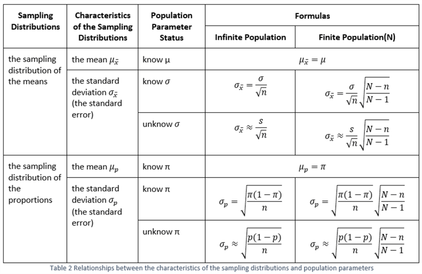
When we select samples of a given size from a population repeatedly, we get different sample statistics. The listing of all values of a sample statistic forms a distribution that is called the sampling distribution of the sample statistics. An example of this is the sampling distribution of the means. Table 2 presents the relationships between the characteristics of a sampling distribution and population parameters. If the population standard deviation is unknown, we can use a sample standard deviation as an unbiased estimator of the parameter. If the population proportion is unknown, we can use a sample proportion as an unbiased estimator of the parameter.
There are two types of parameter estimation: point estimation and interval estimation. The point estimation determines a single value to infer an unknown parameter, and the interval estimation constructs an interval of plausible values for an unknown parameter. The estimation is based on a sample rather than the entire population and thus the mean or proportion of a sample likely differs from the true population mean or the true population proportion. In addition, sample statistics vary from sample to sample. An interval estimate is broader and probably more accurate than a point estimate. The purposes of data analysis have an influence on selecting an estimation type.
1.2 Point Estimation
When we use a sample mean, a sample proportion, and a sample standard deviation to estimate the population mean, the population proportion and the population standard deviation, respectively, we are in each case using a point estimate of the parameter in question [5]. The process of using a sample statistic to estimate the corresponding population parameter is called point estimation, and the value of the statistic is referred to as a point estimate.
To study point estimation via simulation, I installed the database AdventureWorksDW2017 [1]. Then I used the following T-SQL script to select a simple random sample of size 35 from 18,484 customers:
--Use the lottery method to select a SRSWOR of size 35 from this population.
-- https://www.mssqltips.com/sqlservertip/6347/selecting-a-simple-random-sample-from-a-sql-server-database/
CREATE TABLE #lottery_number
(
lottery_numberint primary key
);

--Sample size 35
WHILE (SELECT COUNT(*) FROM #lottery_number) < 35
BEGIN
   BEGIN TRY
      INSERT INTO #lottery_number
      --Select a random [CustomerKey] from 11000 to 29483
      SELECT FLOOR(RAND(CHECKSUM(NEWID())) * (29483 - 11000 + 1)) + 11000
   END TRY
   BEGIN CATCH
      PRINT 'discards duplicates'
   END CATCH
END;

--Store the sample data into a new table SurveyResponse
SELECT [CustomerKey]
      ,[YearlyIncome]
      ,[BikeBuyer]
INTO SurveyResponse
FROM [AdventureWorksDW2017].[dbo].[vTargetMail] c
INNER JOIN #lottery_number l ON c.CustomerKey = l.lottery_number

SELECT * FROM SurveyResponse
DROP TABLE #lottery_number
Table 3 shows a random sample generated by the T-SQL script. I also stored this sample in a database table “SurveyResponse” for future reference. For simulation purposes, I assume this sample data was collected from 35 participants. Each row in the table represents a response from a participant. The first row indicates that the participant reported that his/her yearly income was 70,000 and he/she was not a bike buyer. The second row indicates a response from another participant who was a bike buyer with yearly income 10,000. Other rows contain similar customer information.
| CustomerKey | YearlyIncome | BikeBuyer |
|---|---|---|
| 11254 | 70000 | 0 |
| 11365 | 10000 | 1 |
| 11571 | 30000 | 1 |
| 14202 | 90000 | 0 |
| 14224 | 110000 | 1 |
| 14514 | 30000 | 0 |
| 15098 | 80000 | 0 |
| 15417 | 70000 | 1 |
| 16429 | 30000 | 1 |
| 16946 | 30000 | 1 |
| 17648 | 40000 | 1 |
| 17713 | 10000 | 0 |
| 17924 | 10000 | 1 |
| 18301 | 90000 | 1 |
| 18821 | 80000 | 0 |
| 20146 | 10000 | 0 |
| 20497 | 30000 | 0 |
| 21030 | 30000 | 1 |
| 21518 | 70000 | 0 |
| 21672 | 30000 | 1 |
| 22918 | 80000 | 0 |
| 23453 | 70000 | 1 |
| 23931 | 30000 | 0 |
| 24106 | 30000 | 0 |
| 24532 | 130000 | 0 |
| 24634 | 60000 | 0 |
| 25190 | 60000 | 0 |
| 25907 | 10000 | 0 |
| 26014 | 60000 | 1 |
| 26145 | 70000 | 0 |
| 26490 | 70000 | 1 |
| 27608 | 80000 | 0 |
| 28082 | 100000 | 0 |
| 28297 | 70000 | 1 |
| 28565 | 10000 | 0 |
Table 3 Survey responses from 35 participants
With the sample data in Table 3, we can estimate the population mean by computing the mean of observed values in the sample. Table 1 provides the formula to calculate the sample mean. By using the following equation, the estimate of the mean customer yearly income of the population, which we call a point estimate, is 53714.

To estimate the proportion of bike buyer in all customers, we use the following equation to compute the sample proportion having the characteristic “bike buyer”:
Therefore, the unbiased point estimate of the proportion of bike buyers in all customers is 42.9%.
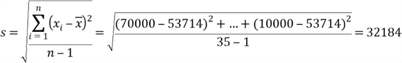
The sample standard deviation is an unbiased estimator of population standard deviation. We calculate the unbiased point estimate by using the formula in Table 1:
The manual calculation process strengthens our understanding of sample statistic computation. There are some other simpler methods. Since I have stored the sample data in the database table “SurveyResponse”, I used the following T-SQL script to compute these point estimates:
SELECT
    AVG(YearlyIncome)           as Mean
   ,1.0*SUM(BikeBuyer)/COUNT(*) as Proportion
   ,STDEV(YearlyIncome)         as [Standard Deviation]
FROM [AdventureWorksDW2017].[dbo].[SurveyResponse]
The Query results shown in the follows are the same as the results of the manual calculation. It is worth noting that there are two standard deviation functions in SQL Server: STDEV and STDEVP [6]. The function STDEV is used to compute statistical standard deviation from sample data, and the function STDEVP is for the population data.
Mean         Proportion       Standard Deviation
53714.2857   0.428571428571   32183.8207695688
Even though a point estimate is able to provide descriptive information about a population, there are some limitations. When we select other samples from the population, we will have different point estimates. Because of random chance, there are some errors in the estimation. In addition, the variation of the difference between a point estimate and the true value of the corresponding population parameter is unknown. Another solution is to construct a confidence interval for the parameter estimation.
1.3 Interval Estimation
The interval estimation approach constructs a confidence interval that likely contains the true value of an unknown parameter. The other important concept in this approach is the confidence level that tells how confident we can be about the interval.
To illustrate the concepts of confidence interval and confidence level, I assume we have already collected yearly income of all customers in the population. I accessed the data through the view “vTargetMail”, and then I knew the population mean 57,306 and standard deviation 32,285. For purposes of illustration, I drew 10,000 random samples of n=35 from the population and computed the mean of each sample. I obtained a list of sample means. Then, I plotted the relative frequency distribution of these sample means shown in Figure 1. The following R script was used to implement the process:
# Reset the compute context to your local workstation.
rxSetComputeContext("local")
# Define connection string to SQL Server
sql.server.conn.string <- "Driver=SQL Server;Server=.;Database=AdventureWorksDW2017;Trusted_Connection={Yes}"
# Create an RxSqlServerData data source object
data.source.object <- RxSqlServerData(sqlQuery = "
                                    SELECT [YearlyIncome] FROM [dbo].[vTargetMail]
                                ",
                                connectionString = sql.server.conn.string)
# Read the data into a data frame in the local R session.
data.frame.yearly.income <- rxImport(data.source.object)
# Initialize a vector for holding sample means
sample.means = rep(NA, 10000)
# Draw samples(n=35) from the population and compute means of the samples
for (i in 1:10000) {
    sample.means[i] = mean(sample(data.frame.yearly.income$YearlyIncome, size = 35, replace = FALSE))
}
# Create a histogram of sample means
hist(sample.means, main = "", xlab = "Sample Mean", freq = TRUE)

Figure 1 The histogram of sample means
According to the approximation form of the central limit theorem (CLT), when the sample size is greater than 30, the sample means are approximately normally distributed even though all these independent observations from a population do not have a normal distribution. Based on the formula in Table 2, the mean of the sampling distribution of the means is computed by:
When the population size N and the sample size n differ by several orders of magnitude, we can ignore the finite correction factor. Therefore, we use the following equation to compute the standard deviation of the sampling distribution:
Figure 2 illustrates the normal distribution N (57306, 54572) that represents the sampling distributions of the means. Because the sampling distribution of the means is normal, 95.45% of sample means lie in the interval [![]() ], i.e. [46392, 68220]. The value of the probability 95.45% is the area under the normal curve over the interval, represented by the grey area in Figure 2. When we expand the width of the interval to [
], i.e. [46392, 68220]. The value of the probability 95.45% is the area under the normal curve over the interval, represented by the grey area in Figure 2. When we expand the width of the interval to [![]() ], i.e. [40935, 73677], the chance of any sample mean being within the interval increases to 99.73%. On the contrary, when we reduce the interval to
], i.e. [40935, 73677], the chance of any sample mean being within the interval increases to 99.73%. On the contrary, when we reduce the interval to ![]() , there is a 68.26% chance that any sample mean lies in this interval.
, there is a 68.26% chance that any sample mean lies in this interval.
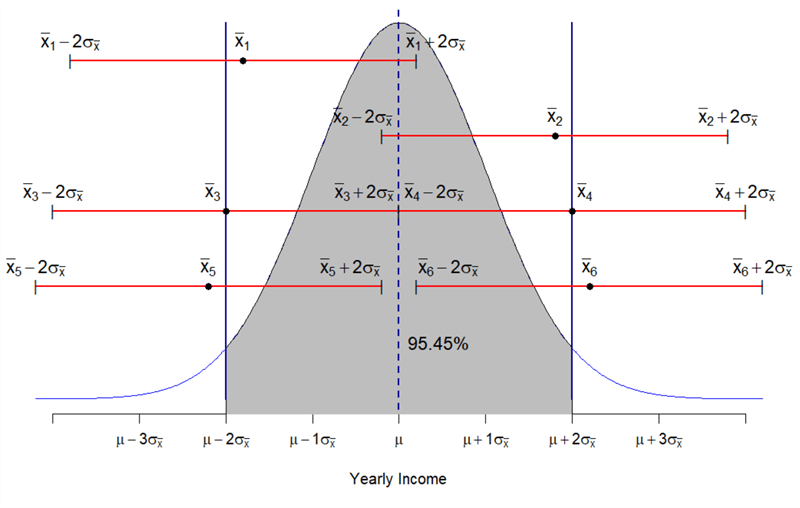
Figure 2 Sampling distribution of the means
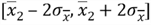
I selected 6 samples and they have sample means ![]() . Then I constructed the intervals
. Then I constructed the intervals ![]() centered at these sample means. These intervals, shown in Figure 2, are defined as follows:
centered at these sample means. These intervals, shown in Figure 2, are defined as follows:
- Interval 1 for sample 1 with mean 47483.4:
 , i.e. [36569.4, 58397.4]
 - Interval 2 for sample 2 with mean 67128.6:
 , i.e. [56214.6, 78042.6]
 - Interval 3 for sample 3 with mean 46392:
 , i.e. [35478, 57306]
 - Interval 4 for sample 4 with mean 68220:
 , i.e. [57306, 79134]
 - Interval 5 for sample 5 with mean 45300.6:
 , i.e. [34386.6, 56214.6]
 - Interval 6 for sample 6 with mean 69311.4:
 , i.e. [58397.4, 80225.4]
Figure 2 reveals that the population mean ![]() lies in the intervals 1, 2, 3, and 4. When a sample mean is less than
lies in the intervals 1, 2, 3, and 4. When a sample mean is less than ![]() or larger than
or larger than ![]() , the intervals constructed by these sample means, such as intervals 5 and 6, do not contain the population mean. We have already stated that there is 95.45% chance that any sample mean falls in the interval
, the intervals constructed by these sample means, such as intervals 5 and 6, do not contain the population mean. We have already stated that there is 95.45% chance that any sample mean falls in the interval ![]() . Thus, in the long run, for all intervals constructed by
. Thus, in the long run, for all intervals constructed by ![]() , 95.45% of them contain the population mean. If I draw 10,000 samples from the population and construct 10,000 intervals
, 95.45% of them contain the population mean. If I draw 10,000 samples from the population and construct 10,000 intervals ![]() , about 9545 intervals may contain the population mean. The interval
, about 9545 intervals may contain the population mean. The interval ![]() is called a 95.45% confidence interval and the percentage is called confidence level. The decimal value of the percentage, i.e. 0.9545, is called confidence coefficient. Notice that the confidence interval varies from sample to sample.
is called a 95.45% confidence interval and the percentage is called confidence level. The decimal value of the percentage, i.e. 0.9545, is called confidence coefficient. Notice that the confidence interval varies from sample to sample.
To estimate the value of a population parameter, we construct an interval centered at the corresponding sample statistic in such a way that we can be confident that the interval contains the true value of the parameter. This process is called interval estimation. If sample 1 is selected to estimate the mean of the population, the 95.45% confidence interval for the population mean is [36569.4, 58397.4]. That is to say, we are 95.45% confident that the true mean is between 36569.4 and 58397.4.
2 – Large-Sample Confidence Interval for the Population Mean
In this tip, we want to estimate the mean value of the yearly income of all customers. To solve this problem, we have selected 35 participants randomly who reported their yearly incomes and told whether they owned a bike. The sample data is shown in table 3. I have already saved these data in the database table “SurveyResponse”. Then, let’s follow these steps to construct a 95% confidence interval for the population mean of customer yearly incomes:
Step 1: Find the sample size, the sample mean, and the standard error of the sample mean.
We have already computed these values in Section 1:
Sample size ![]()
Sample mean ![]()
The standard error of the sample mean ![]()
Step 2: Compute the z-score.

Step 3: Obtain a 95% confidence interval for the z-score by using the standard normal table.
Plug the z-score into the inequality:
Step 4: Construct a 95% confidence interval for the population mean by solving the inequality.
The interval [43018.28, 64409.72] is called a 95% confidence interval for the population mean. We can be 95% confident that the interval [43018.28, 64409.72] contains the true mean.
In the 4-step process, the standard normal table was used to find the critical value of z score. R language provides commands to find the confidence interval:
# Reset the compute context to your local workstation.
rxSetComputeContext("local")
# Define the connection string to SQL Server
sql.server.conn.string <- "Driver=SQL Server;Server=.;Database=AdventureWorksDW2017;Trusted_Connection={Yes}"
# Create an RxSqlServerData data source object
data.source.object <- RxSqlServerData(sqlQuery = "
                                    SELECT [YearlyIncome] FROM [dbo].[SurveyResponse]
                                ",
                                connectionString = sql.server.conn.string)
# Read the data into a data frame in the local R session.
data.frame.yearly.income <- rxImport(data.source.object)
# Define a vector for holding sample data
yearly.income = data.frame.yearly.income$YearlyIncome
# Write down known values
sample.size <- 35
population.standard.deviation <- 32285
sample.mean <- mean(yearly.income)
confidence.interval <- 0.95
# Compute the standard error
standard.error <- population.standard.deviation / sqrt(sample.size)
# Find the critical value of z score
alpha <- 1 - confidence.interval
z.alpha <- qnorm(1 - alpha/2)
# Compute the margin error
margin.error <- z.alpha * population.standard.deviation / sqrt(sample.size)
# Construct the confidence interval
lower.limit <- sample.mean - margin.error
upper.limit <- sample.mean + margin.error
# Print the result
sprintf('The %d%% confidence interval for the population is [%.2f, %.2f]',
        confidence.interval*100, lower.limit, upper.limit)
The results shown in the following are almost the same as the estimation by the manual process. The manual calculation strengthens our understanding of interval estimation. We usually use modern data analytic tools, for example, Python, R, and SAS, to construct a confidence interval.
[1] "The 95% confidence interval for the population is [43018.45, 64410.12]"
3 – Large-Sample Confidence Interval for the Population Proportion
We also want to estimate the proportion of bike buyers in all customers from a sample. Here, we estimate the percentage (or proportion) of some groups with a certain characteristic [7]. When a sample unit has a certain characteristic, we consider the unit having an outcome of success. On the other side, any sample unit that does not have the characteristic is considered to have an outcome of failure. Consequently, any sample unit has two outcomes: success and failure. We can think of the sample as a collection of outcomes from an experiment that repeats the Bernoulli trial 35 times. Therefore, the sampling distribution of the proportions is a binomial distribution.
We can use a normal distribution to approximate a binomial distribution. Bagui and Mehra presented four different proofs of the convergence of binomial distribution to a limiting normal distribution when the number of trials approaches infinity [8]. In practice, we use a normal distribution to approximate a binomial distribution when the number of trials is greater than 30.
In addition, we study the sample proportion from a different perspective. If we consider the outcome success to be value 1 and consider the outcome failure to be value 0, the mean is the proportion of all outcomes who are successes, i.e. the proportion of bike buyers. Then, we can apply the approximation form of the central limit theorem (CLT). When the sample size is greater than 30, the sample proportions are approximately normally distributed.
Thus, for a large sample (n>30), the sampling distribution of the proportions approximates to a normal distribution and we are able to use the properties of normal distribution [2]. Let’s construct a 95% confidence interval for the proportion of all customers who are bike buyers:
Step 1: Find the sample size, the sample proportion and the standard error of the sample proportion.
We have already computed these values in Section 1:
Sample size ![]()
Sample proportion ![]()
Since the population proportion π is unknown, we use the sample proportion p as an unbiased estimator to calculate the standard error. When the size of the population and the sample size differ by several orders of magnitude, we can ignore the finite correction factor. Therefore, we use the following equation to compute the standard deviation of the sampling distribution of the proportions:

Step 2: Compute the z-score.

Step 3: Obtain a 95% confidence interval for the z-score by using the standard normal table.
Plug the z-score into the inequality:
Step 4: Construct a 95% confidence interval for the population proportion by solving the inequality.
The interval [0.265, 0.593] is called a 95% confidence interval for the population proportion. We can be 95% confident that the percentage of all customers who are bike buyers is between 26.5% and 59.3%.
I would like to point out that I use the properties of a normal distribution to construct the interval only when the sample size n is large than 30. Some data analysts may check other conditions, for example, ![]() and
and ![]() [8].
[8].
4 – Parameter Estimation for Small Samples (n≤30)
In practice, we may not always have a large sample. When we use a small sample that the size of the sample is less than or equal to 30 to make inferences about population parameters, we have two immediate problems [7]:
- The sampling distribution of means may not approximate normal;
- When the population standard deviation is unknown, the sample standard deviation may not approximate the population standard deviation;
To solve these two problems, we use Student’s t-distribution [9]. Instead of calculating the z-statistic, we use the following equation to compute the t-statistic:

The t-distribution looks like a normal distribution, but it has heavier tails and flatter central region. The study of Student’s t-distribution could be worth another tip. I am going to use an example to show the process of construction of a confidence interval from a small sample. Professor Jost provided a dataset that contains thicknesses of a piece of white paper [10]. Table 4 shows the 27 measurements observed from a micrometer. Let’s continue to follow the 4-step process to find a 95% confidence interval for the true thickness.

Step 1: Find the sample size, the sample mean and the sample standard deviation.
Since we have already known the computation of sample size, the sample mean and the sample standard deviation, I used the following R script to compute these values:
sample.data <- c(0.098, 0.110, 0.099, 0.107, 0.102, 0.102, 0.095, 0.105, 0.101,
                 0.101, 0.106, 0.101, 0.105, 0.104, 0.107, 0.101, 0.098, 0.104,
                 0.106, 0.104, 0.100, 0.104, 0.106, 0.102, 0.106, 0.104, 0.105)
sprintf('sample size %d', length(sample.data))
sprintf('sample mean %f', mean(sample.data))
sprintf('sample standard error %f', sd(sample.data))
The script printed out the results as follows:
[1] "sample size 27"
[1] "sample mean 0.103074"
[1] "sample standard error 0.003350"
Thus, we have known these values:
Sample size ![]()
Degrees of freedom ![]()
Sample mean ![]()
Sample standard deviation ![]()
Step 2: Compute the t-statistic.
Since the sample size is less than 30, we use t-distribution with 26 degrees of freedom:
Step 3: Obtain a 95% confidence interval for the t-statistic by using the t-distribution table.
Plug the t-statistic into the inequality:
Step 4: Construct a 95% confidence interval for the population mean by solving the inequality.
Round to four decimal places:![]()
![]()
The interval [0.1017, 0.1044] is called a 95% confidence interval for the population mean. We are 95% confident that the interval [0.1017, 0.1044] contains the true thickness.
To verify this manual calculation, I used the “t.test” command provided by R language to get a 95% confidence interval for the population mean. In the existing R session, I executed the command “t.test(sample.data, conf.level = 0.95)” in the “R Interactive – Microsoft R Client(3.4.3.0)” window. The following output from the interactive window reports the 95% confidence interval for the population mean is [0.1017487 0.1043994]. The result from the “t.test” command agrees with the manual calculation result.
> t.test(sample.data, conf.level = 0.95)

   One Sample t-test

data:  sample.data
t = 159.86, df = 26, p-value < 2.2e-16
alternative hypothesis: true mean is not equal to 0
95 percent confidence interval:
 0.1017487 0.1043994
sample estimates:
mean of x
0.1030741

>
Guttman and Gupta [11] remind that the population should be normal or approximately normal when we use Student's t-distribution to construct a confidence interval to estimate the population mean from a small sample (n<30). However, other textbooks, for example [2], don’t have this kind of reminding.
Summary
We started the tip with a problem statement that data analysts would like to estimate population parameters from sample statistics. The solution is to construct a confidence interval within which the population parameter lies. The techniques involved in this solution can be used to estimate the population mean and the population proportion.
After an overview of the unbiased estimators: sample mean, sample proportion and sample standard deviation, we have presented relationships between the characteristics of the sampling distributions and population parameters. Then, we have introduced two approaches to make an inference about the population from sample data: point estimation and interval estimation. The point estimation is to use a single value of a statistic as an estimate of a population parameter. The interval estimation is to construct a confidence interval from the sample data and the population parameter lies in the interval with a certain level of confidence.
While introducing the techniques of parameter estimation, I explained the concepts of the confidence interval and the confidence level. The approximation form of the central limit theorem (CLT) enables us to construct a confidence interval for a large sample by using normal distribution properties.
We then constructed a confidence interval centered at the mean for a large sample (n>30) when we knew the population standard deviation. We also discussed a technique that finds a confidence interval of proportion for large samples (n>30) when the population proportion is unknown.
Finally, we glanced at the small samples (n≤30). While we cannot ensure the sampling distribution of the means is approximately normal, we used Student’s t-distribution to find the confidence interval.
References
[1] Kess, B. (2017). AdventureWorks sample databases. Retrieved from https://github.com/Microsoft/sql-server-samples/releases/tag/adventureworks/.
[2] Hummelbrunner, S. A., Rak, L. J., Fortura, P., & Taylor, P. (2003). Contemporary Business Statistics with Canadian Applications (3rd Edition). Toronto, ON: Prentice Hall.
[3] Black, K. (2013). Business Statistics: For Contemporary Decision Making, 8th Edition. Hoboken, NJ: Wiley.
[4] William, M., & Sincich, T. (2012). A Second Course in Statistics: Regression Analysis (7th Edition). Boston, MA: Prentice Hall.
[5] Miller, I., & Miller, M. (2012). John E. Freund’s Mathematical Statistics with Application (8th Edition). Essex, UK: Pearson.
[6] Ayyappan. (2013). SQL SERVER – Standard deviation functions STDEV and STDEVP – @SQLSERVER: https://sqlserverrider.wordpress.com/2013/03/06/standard-deviation-functions-stdev-and-stdevp-sql-server/.
[7] Sincich, T. T, & McClave, T. J. (2016). A First Course in Statistics 12th Edition. Boston, MA: Pearson.
[8] Bagui, S. & Mehra, L. K. (2017). Convergence of Binomial to Normal: Multiple Proofs. International Mathematical Forum, Vol. 12, 2017, No. 9, 399-411.
[9] Hwang, J. & Blitzstein, K. J. (2015). Introduction to Probability. Boca Raton, FL: CRC Press.
[10] Jost, S. (2017). CSC 423: Data Analysis and Regression. Retrieved from DePaul University Website: http://facweb.cs.depaul.edu/sjost/csc423/
[11] Guttman, I., & Gupta, C. B. (2013). Statistics and Probability with Applications for Engineers and Scientists. Hoboken, NJ: John Wiley & Sons.
Next Steps
- When we get a 95% confidence interval for the true mean, we should correctly interpret the interval. A typical misconception interprets that there is a 95% chance that the true population mean falls within the confidence interval. The confidence interval not only gives a range but reveals how stable the estimate is. We cannot guarantee that a single sample represents the population. The true mean may not be in the interval constructed by a sample. We use a value of confidence level to describe the uncertainty associated with the estimation process. A confidence level, for example, 95%, means that, by running the process repeatedly, we get many computed intervals, and 95% of these intervals contain the true mean. Thus, the correct interpretation is that we are 95% confident that the interval contains the true population mean.
- Check out these related tips:

Nai Biao Zhou has twenty years of experience in software development, with strong analytical skills and a broad range of computer expertise.
He has fifteen years of experience in development and maintenance of database applications on SQL Server in OLTP/OLAP/BI environments.
He has a master’s degree in Control Engineering and is pursuing a Master of Science degree in Predictive Analytics.
Knowledge/Skills
Advanced computer programming skills and well versed with C/C#, Java, ASP.NET, JavaScript, and SQL.
In depth knowledge of Solution Architecture, and Software Development Life Cycle (SDLC).
Microsoft Certified Application Developer (MCAD) since 2004.
- MSSQLTips Awards: Author of the Year – 2021 | Rising Star (50+ tips) – 2024 | Author Contender – 2020, 2023


