Data Science for Inferential and Predictive Statistics

By: Rick Dobson | Comments | Related: More > Data Science

Problem

I am a SQL professional who seeks a Data Science overview to increase my capabilities for analyzing with inferential and predictive statistics existing data on my database servers.

Solution

This tip is a follow-up to an earlier one that introduced core data science disciplines with specific examples of how they could be performed via SQL programming skills. The earlier tip focused on prior SQL code demonstrations for performing data science techniques. This tip switches the focus to data science applications for which prior SQL code demonstrations are not commonly available but for which SQL is fully capable of addressing.

Data science depends on programming (loosely interpreted), data analysis and modeling, and substantive knowledge in a domain. SQL professionals typically have much experience in managing data, and data applications are a core focus for data science. Therefore, it is efficient for SQL professionals to participate meaningfully in data science projects. Additionally, SQL has programming capabilities to enable the performance of many data science activities -- one especially easy step is to analyze existing data on database servers managed and used regularly by SQL professionals.

This tip begins with a focus on how statistics can be programmed via SQL to infer which differences count the most and what models are best for use in data science projects. This initial exposure leverages a prior tip on a SQL starter statistics package by suggesting package additions. The overview in this tip sketches out next steps to expand the scope of the starter package towards a full-fledged SQL statistics package that will empower SQL professionals to easily and cost efficiently make significant contributions to data science projects. The Next Steps section closes the tip with a compilation of references cited from within this tip as well as a worksheet download link for referenced worksheets.

A quick review of the SQL starter statistics package

A key objective of the SQL starter statistics package is to provide a framework for implementing statistics in data science projects. Because the package is implemented via a collection of stored procedures, the package is easy for SQL professionals to start using. The stored procedure for each test or collection of tests requires the migration of data into one or more temporary tables on which the stored procedures operate to perform a statistical operation.

The initial starter package covered both descriptive, inferential, and predictive statistics. The starter package presents each statistics technique from two perspectives. First, how to use the technique as it is implemented in the package. Second, understanding when and how to use statistics implemented by each stored procedure. Here's a top line summary of statistics already in the existing starter package.

Overall median and median by group
Coefficient of determination
Fitting a line to a set of data
t tests for computing that statistical difference between sets of measurements

This tip begins by examining several areas for growing the starter package. Each area is selected because of its relevance to data science. You are invited to propose additional areas for augmenting the initial SQL starter statistics package. Just leave a comment to this tip with any areas beyond those mentioned in the remaining sections of this tip.

Prospective t test features for the SQL statistics package

The purpose of this section is to briefly describe a collection of new and supplementary capabilities for t tests in a future version of the SQL statistics package.

The SQL starter statistics package version 1.0 introduced the capability to perform two types of t tests. The first test was for the difference in the means between two groups. While it was not explicitly mentioned, the two groups were assumed to have the same sample size and variance. The second test was a repeated measures test where the same entities were tested with two different treatments. The t test was for the mean of the differences between all the entities being tested with two treatments or conditions. The starter package required users to look up the calculated t value for each kind of test in a table of critical t values.

Many statistical procedures, including t tests, are for the selection of a null hypothesis versus an alternative hypothesis; t tests frequently involve the comparisons of means between two groups, but the groups need not necessarily have the same sample size and variance. The null hypothesis is normally specified so that you can reject it at a specified probability level and thereby accept the alternative hypothesis.

If it only matters that two groups are different but not that one group in particular is greater than another group, then you can perform a two-tailed test.
- The null hypothesis would be for the sample means to equal one another.
- The alternative hypothesis would be for the sample means to not equal one another.
If it does matter whether the results in one sample are greater than another sample, then you can perform a one-tailed test.
- The null hypothesis would be for one sample mean to be less than or equal to the mean for a second sample.
- The alternative hypothesis would be for one sample mean to be greater than another sample mean.

According to Wikipedia, there are four types of t tests for the difference between two independent group means or one group mean and a specified value.

The one-sample t test compares a sample mean to a specified value. If the sample mean is represented by x-bar, the specified value is represented by mu sub-zero, and the sample standard deviation is represented by s, then you can use the following expressions to calculate a t value. The degrees of freedom for the calculated t value is n - 1 where n is the sample size.
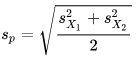
The independent two-sample t test with the sample size and sample variance in both groups being the same can be calculated with the following expressions. This is one of the two t tests included in the SQL starter statistics package. The group means are X-bar₁ and X-bar₂. The pooled standard deviation is Sp. The sample variances for the first and second groups are, respectively, S² sub-X₁ and S² sub-X₂. The degrees of freedom for the calculated t value is 2n - 2 where n is the sample size per group.
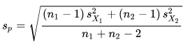
The independent two-sample t test with equal or unequal sample size and the same sample variance in both groups is a third type of t test. The calculated t value for this type of t test relies on the next two expressions. The group means are X-bar₁ and X-bar₂. The pooled standard deviation is Sp. The sample variances for the first and second groups are, respectively, S² sub-X₁ and S² sub-X₂. The degrees of freedom for the calculated t value is (n1 + n2 -2) where n1 and n2 are sample sizes for the first and second groups.
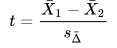
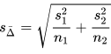
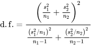
The independent two-sample t test only for use with unequal sample variances in both groups is a fourth type of t test; this test is sometimes referred to as Welch's t test. The calculated t value for this type of t test relies on the next two expressions, and the degrees of freedom for the calculated t value is denoted by the third expression. The group means are X-bar1 and X-bar2. The sample variances in the first and second groups are S₁ and S₂. The sample sizes in the first and second groups are n1 and n2. Notice that the denominator for the calculated t value is not a pooled variance, this is why the degrees of freedom expression for this test involves both sample sizes and sample variances.

Wikipedia also references a fifth kind of t test for the difference for two sets of repeated measures on the same set of entities or when two independent samples have been matched on a variable. This t test is called the dependent t test for paired samples test. The repeated measures version of this test is the second of two t tests in the SQL starter statistics package.

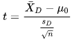
The dependent t test for paired samples is based on the sample mean difference (X-bar_D) and the sample standard deviation of the differences (S_D). When you just want to test the null hypothesis of no difference between the two sets of repeated measures, then mu sub-zero can be ignored or omitted. Otherwise, specify a value for mu sub-zero. With a non-zero mu sub-zero, you are able to reject the hypothesis that the difference between the means is some specific non-zero value.

For example, a data scientist may want to know if two different models are generating different outcomes. There is no a priori assumption about which model is better. If this is the case, the null hypothesis could be that there is no difference in the mean change between the two models. On the other hand, if we were testing for a new miracle compound that was being tested to generate a fifty-percentage point gain over some standard compound routinely being used, then we could test for differences with mu sub-zero equal to fifty percentage points greater than for the standard compound routinely being used.

To assess if a calculated t statistic is significant for any given set of data, you need to consult a critical t values resource for a degrees of freedom and the kind of difference that matters (two-tailed or one-tailed). It is typical to designate statistical significance at one of several probability levels, such as less than or equal to five per cent (.05), one per cent (.01), or one-tenth of one percent (.001).

In the tip describing the SQL starter statistics package, users of either of the two t tests were advised to consult a table of critical t values from the NIST/SEMATECH e-Handbook of Statistical Methods. However, you can use Excel built-in functions for returning t critical values that are suitable for evaluating if a calculated t value with a specified degrees of freedom is statistically significant for either a one-tailed or a two-tailed test.

Use the T.INV.2T function for a two-tailed test. The function takes two parameters for probability level and degrees of freedom and returns a critical t value. If the calculated t value is more positive than the returned value or more negative than -1 times the returned value, the calculated t value is statistically significant for a two-tailed t test with the designated degrees of freedom and probability level.
Use the T.INV function for a one-tailed test. This function also takes parameters for the probability level and degrees of freedom and returns a critical t value. Wrap the return value from the function in an absolute value function and do the same for the calculated t value. If the absolute value of the calculated t value exceeds the absolute value of the critical value, then the calculated t value is statistically significant for a two-tailed t test with the designated degrees of freedom and probability level.

The following screen shot shows the instructions and an excerpt from the table of critical t values from the NIST/SEMATECH e-Handbook of Statistical Methods. Instructions for how to derive critical t values for one-tailed and two-tailed t tests precede the table. Two values are highlighted by red boxes.

The 2.764 value is the critical t value for the .01 probability (or alpha) level with a one-tailed t test with ten degrees of freedom.
The 3.169 value is the critical t value for .01 probability (or alpha) level with a two-tailed t test with ten degrees of freedom.

The next screen shot shows an excerpt from an Excel workbook populated with return values for the T.INV.2T and T.INV functions for critical two-tailed and one-tailed t values respectively. The two-tailed values are in cells B3 through D14. The one-tailed critical t values are in cells F3 through H14.

The screen shot below shows the cursor resting in cell C12. The T.INV.2T function in this cell references the degrees of freedom in cell A12 and the probability of alpha level in cell C2. The value in cell C12 matches the two-tailed critical t value for ten degrees of freedom in the preceding table.
The matching one-tailed critical t value for ten degrees of freedom at the .01 probability or alpha level appears in cell G12. This value shows as 2.764, but the expression returning the value does not show because the cursor was resting in cell C12 when the screen shot was taken. However, the expression for generating the one-tailed value in cell G12 is =ABS(T.INV(G$2,$A12)).
For your convenience, the worksheet file with the expressions for all cell values showing in the screen shot below is available for download with this tip.

Many SQL professionals are adept at loading data from an Excel workbook file into a SQL Server table. By populating separate tables of critical t values into an Excel table, you can then load into SQL Server from Excel one-tailed and two-tailed tables of critical values. Then, you can revise the stored procedures for computing calculated t values so that they report the calculated t value, its degrees of freedom, whether the calculated t value is statistically significant, and if so, at what level you can reject the null hypothesis. This would eliminate the need to consult a resource of critical t values to assess the probability of a calculated t value.

Adding F test capabilities to the SQL statistics package

Another direction for enhancement of the SQL statistics package is to add new kinds of statistical tests that are of a different kind than t tests. After all, t tests mostly center on determining if any difference is statistically significant between two sets of measurements for independent groups or two sets of repeated measures for a single group. In some cases, you may have measurements for more than two groups. For example, you may want to know if the close price change is significantly different for stocks with large, mid-sized, or small capitalizations. This question involves comparing three groups instead of just two groups. You can use a one-way F test defined as the ratio of variances for assessing if stock capitalization affects mean change in close price.

You may even want to know does change in close price vary significantly by both stock capitalization and stock sector. In this case each stock is categorized by both stock capitalization and sector. For this reason, an F test for this kind of comparison is known as a two-factor design. In addition to the main effect for each factor, you can also use an F test to assess the interaction between factors on the dependent variable. The F test is designed to facilitate these kinds of comparisons.

The F test is often referred to as an analysis of variance (ANOVA) test. This is because the F test depends on a ratio of variances. The variances are the deviations of the response variable, such as stock close price change, for different levels within a factor. The levels can be defined by quantitative values, such as small, medium, and large capitalization, or merely present or not, such as whether a stock is in the Information Technology sector or not. The ANOVA test results allows you to make assertions about the statistical significance of differences within and across levels within factors.

For a one-factor or one-way ANOVA,
- The null hypothesis is that there is no difference between the means across levels
- If you are able to reject this hypothesis, then you can accept the alternative hypothesis that the means are not the same across all levels of one factor
For a two-factor or two-way ANOVA, there are three null hypotheses with matching alternative hypotheses.
- The null hypothesis for the first factor is that there are no significant differences between the means for its levels. The alternative hypothesis for the first factor is that the mean for at least one of its levels is different than the means for the remaining levels.
- The null hypothesis for the second factor is that there are no significant differences between the means for its levels. The alternative hypothesis for the second factor is that the mean for at least one of its levels is different than the means for the remaining levels.
- There is also a null hypothesis that there is no interaction effect. If you can reject this null hypothesis, then you accept the alternative hypothesis that there is a statistically significant interaction effect for the interaction of levels between the two factors.

The variances that are compared are for differences of individual scores within the levels for a factor to the means within levels for a factor. The overall computational guidelines for ANOVA tests partitions variances by levels within factors, interaction effects, and residual error. The residual error is the individual score variance that cannot be credited to main factor effects or interaction effects.

If you want to forge ahead with ANOVA testing before it is incorporated into a future version of the SQL statistics package, you can learn about the detailed computational guidelines from section 7.4.3 in the NIST/SEMATECH e-Handbook of Statistical Methods. It is one of the best sources that I found for clearly and concisely explaining how to perform the calculations for F tests.

Just as with the t test, there is an Excel function for denoting the critical F test values. If you populate a SQL Server table with values from the function, then you can look up the probability level associated when a calculated F test value exceeds a critical F test value. This probability is the statistical significance associated with the calculated F test value.

Adding Chi Square test capabilities to the SQL statistics package

Both the t test and the F test process scaled data as a dependent variable, but you may sometimes need to determine if observed counts by bin are significantly different from expected counts by bin. The Chi Square test aims to serve this role. The observed frequencies may be derived from a contingency table in which entities, such as stocks, persons or even just incidents, are classified relative to row and column categorical identifiers. At other times, the observed frequencies might be the probability or cumulative probability that observed counts fall within a set of category ranges sometimes called bins. In these cases, you can compare an observed set of frequencies to a normal probability density function or a normal cumulative density function. Of course, you can use any functionally specified distribution, such as binomial, Poisson, exponential, or hypergeometric where one of these distributions model an empirical distribution that you are studying with a data science project. However, this section focuses on the difference between observed and expected frequencies within a contingency table.

This section focuses on the Chi Square test for homogeneity and the Chi Square test for independence. Both tests start with a set of observed frequencies from a contingency table. However, the way the table is populated, and the interpretation of the results are different depending on the test. Nevertheless, the computational details of both tests are exactly the same.

The Chi Square Test for independence measures the degree of association between two categorical variables from the same population.
The Chi Square test for homogeneity assesses if a categorical variable is distributed in the same proportion of counts across two or more different populations.

Both tests rely on a contingency table, such as the one showing in the screen shot below for observed counts.

The contingency table has n rows and n columns. Please keep in mind that the number of rows and columns for a contingency table are not required to be the same.
The count in each cell of the table is denoted by count _ri,cj where values of i and j extend from 1 through n.
The minimum frequency for any cell of the contingency table should be five -- otherwise the Chi Square test results are not reliable. In this case, you can simply re-specify the row and column categories so that no cell has an observed frequency of less than five.
Below and to the right of the contingency table columns and rows, there are sums of column and row counts. Column 1 Count denotes the sum of the cell counts in the first column. Similarly, Row 1 Count denotes the sum of the cell counts in the first row.
The sum of the counts across all contingency cells is denoted by Grand Count; this cell is below and to the right of the contingency table.
As indicated above, both the independence test and the homogeneity test use a contingency table like the one showing below, but the rows and column values are specified differently.
- In the test for independence, the rows and columns designate different variable values - one set of categories for the rows and another set of categories for the columns. Two examples of continuous stock domain variables that can be split into categories are average daily volume and stock share price.
- In the test for homogeneity, the rows identify different samples, such as Dow Jones, NASDAQ 100, and the Russell 2000 stock index averages. The columns denote a categorized variable, such as a grouping for the number of trading days in the past year during which an index increased from the preceding trading day.

The next screen shot shows the expressions for calculating expected frequencies based on independence between row and column identifiers for the contingency table. The Chi Square test compares the observed counts to the expected frequencies. You are not required to use expected frequency expressions based on independence, but this assumption works well for both the independence and homogeneity tests. With expressions for expected frequencies based on independence, you can reject

the null hypothesis of no difference between the populations for the test of homogeneity
the null hypothesis of no association between the category variables for the test of independence

The next screen shot shows how to use the Observed Counts and Expected Counts tables to compute a calculated Chi Square value that measures the statistical significance of the difference between the two sets of frequencies.

The process starts creating a new table with the same number of rows and columns as in the original Observed Counts table.
Next, each cell within the new table is populated by the squared difference of the observed cell value less the expected cell value divided by the expected cell value.
Lastly, the calculated Chi Square value is computed by taking the sum of all the calculated cells in the new table.
The expressions for a populated version of the table appear in the following screen shot.

The computational steps, which are described in detail above, generate a calculated Chi Square component value for each cell in a contingency table. Columns B through F in the screen shot below contain the expressions that facilitate the computing of independence for row and column variables.

Cells C4 through E6 contain the original observed cell counts. You can copy into these cells either of two source contingency tables.
- Cells L4 through N6 contain a table for which you cannot reject the null hypothesis of independence for row and column counts.
- Cells L16 through N18 contain a table for which you can reject the null hypothesis of independence for row and column counts.
Cells C13 through E15 show the expected frequencies for the observed row and column counts in cells C4 through E6. Expressions within these cells (C13:E15) compute the values that show.
Cells C20 through cells E22 show the Chi Square component value for a cell based on the observed and expected frequencies. These cells contain expressions for the squared deviation of the expected frequency from the observed frequency divided by the expected frequency. Below this final table on the left side are three more rows.
- The first row shows the calculated Chi Square value, which is merely the sum of cells in the table above it.
- The second row shows the degrees of freedom, which is the number of rows less one multiplied by the number of column less one; this is two times two in our example.
- The third rows shows the output from the Excel CHISQ.DIST.RT function ( here and here). This function returns the probability of obtaining a calculated Chi Square value by chance from the Chi Square cumulative distribution function. The function takes two values:
  - Calculated Chi Square value (or any arbitrary value for Chi Square)
  - Degrees of freedom
- For the original counts showing in cells C4 through E6, the probability of this distribution occurring by chance is less than .01; more precisely, the probability is .008642 rounded to six places after the decimal point.
The worksheet tab comes equipped for easy testing of the independence null hypothesis.
- Cells L4 through N6 contains a contingency table in which the null hypothesis of independence cannot be rejected. The three rows below the matrix contain the literal outcome values for the contingency table.
- Cells L16 through N18 contains a contingency table in which the null hypothesis of independence can be rejected. The three rows below the matrix contain the literal outcome values for the contingency matrix.

The Chi Square table for homogeneity tests between two variables from the same sample of entities to see if the two variables interact with one another. That is, if you know the value for a row category variable can you estimate the corresponding column category variable value(s). The two variables are either naturally categorical or non-categorical with boundaries values specified for row and/or column variables to force observations into categories.

Adding matrix processing capabilities to the SQL statistics package

If you want to use SQL to program more than two independent variables to estimate a dependent variable, then you need a matrix algebra capability and the ability to compute determinants from within SQL. This section explains why and introduces key concepts for multivariate regression. A follow-up set of tips will dive more deeply into the topic by comparing implementation strategies - at least one of which will be incorporated into a subsequent SQL statistics package version. Also, the processing of matrices with SQL will eventually prove useful for principal components analysis., which is another multivariate analysis technique that complements multivariate regression.

A helpful introduction to multiple linear regression for two independent variables is available from professor Michael Brannick; you may recall him as the author who presented a solution framework and sample data that served as a model for the single variable regression solution in the SQL starter statistics package. Professor Brannick's two-variable model for multivariate regression appears in a paper posted on a website from the university of South Florida. He provides the theory, computational expressions, and a fully worked example for how to estimate a dependent variable from two independent variables. The general equation that he solves for has the form shown below. Y' is the estimated dependent variable value. The b₁ and b₂ values are regression coefficients for estimating Y' for Y, the observed dependent variable value, and a is a constant for the location of the equation within the X1, X2, and Y coordinate system.

The general equation allows for more than two independent variables by reference to the b3 through bk coefficients and the X3 through the Xk independent variable values. However, professor Brannick's paper never addresses more than two independent variables, except for referring the reader to a solution based on matrix algebra. I was unable to discover his expressions for implementing the matrix algebra solution. This tip includes references for implementing matrix algebra solutions via SQL. Future tips will test the practical utility of these references for facilitating the implementation of multivariate regression for more than two independent variables.

Professor Ezequiel Uriel Jimenez of the University of Valencia in Spain takes a matrix algebra approach to multivariate linear regression . His orientation is from the perspective of econometrics, and it is not primarily computational in its presentation. However, he clearly identifies the data sources and computed values from a matrix algebra orientation.

Professor Jimenez starts with a y vector of n values and an X matrix of with n rows and k columns. The y values represent the observed dependent variable values, and the X matrix elements represent independent variable values plus one more column for a constant, such as the a in professor's Brannick's paper. The variable n represents the units over which regression extends. For example, if you estimated advanced database programming grades for a set of 100 students, then n would equal 100, and each student's grade would represent a different element in the y vector. The first column in the X matrix is for the regression constant. The values x_2,1 through x_k,1 are for the independent variable scores for the first of one hundred students; the independent variable values could include values such as IQ, mathematics SAT or ACT scores, and grades from an introduction to database programming course.

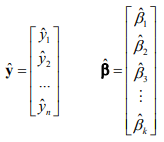
Two additional vectors facilitate a matrix algebra representation of the expression for the set of estimated student grades (y-hat) from the X matrix. The y-hat vector has the same shape and number of elements as the y vector; the y-hat vector has estimated values for the elements in the y vector. The beta-hat vector is a column vector of k elements - one for the regression constant and one for each independent variable.

After designating these matrix algebra components, you can specify the expression for the y-hat elements with the following matrix algebra equation. The X matrix post multiplied by the beta-hat vector follows the rules of matrix multiplication. Basically, the row elements of the X matrix are multiplied by the elements of the beta-hat vector and summed to calculate the estimated grades (y-hat row values); each row in X is for an element in y-hat. Because there are one hundred rows and k columns in the X matrix and k elements in the beta-hat vector, there are one hundred y-hat elements.

Given the preceding equation and assumptions about the distribution of residuals between y elements less y-hat elements, professor Jimenez designates the ordinary least squares (OLS) estimates of the beta-hat elements with the following equation. The term X' denotes the transposition of the X matrix; this is the ninety-degree clockwise rotation of the elements in X. The X'X expression represents the post multiplication of the transpose for the X matrix multiplied by the X matrix. The negative power of one for the [X'X] matrix denotes the inverse of the [X'X] matrix. When matrix A is multiplied by its inverse, then the resulting matrix is the identity matrix (one values in the central upper-left to bottom-right diagonal elements and zeroes elsewhere).

In order to calculate a result based on professor Jimenez's formulation, we need SQL code for

representing matrix and vector elements in SQL tables
deriving a transposed matrix from an original matrix
implementing matrix multiplication
computing the inverse of a matrix

I was able to find the first three elements of the solution within SQL in the following two references from Joe Celko and Deirdre O'Leary. Joe's paper is wider in scope and offers special code for computing with SQL the transpose of a matrix. Both papers rely on the same scheme for representing a matrix in a SQL table and performing matrix multiplication, but the Deidre O'Leary reference may be a little clearer for those who have less familiarity with matrix algebra.

There is one solution element for which I was not able to find a general prior reference with SQL guidelines on how to implement the element. This is the computation of the inverse of a matrix. However, I did discover some code at sqlfiddle.com on how to compute an inverse for a square matrix with two rows and two columns. Expanding this example to a matrix of indefinite size of even to three-by-three and four-by-four matrices may be non-trivial for some SQL developers.

There are at least two popular approaches to computing the inverse of a matrix. Both approaches rely on the computation of a determinant for a matrix that is then multiplied by the matrix to derive its inverse. Wikipedia offers introductions to the mechanics of both approaches. One method depends on Gaussian elimination, and the other method depends on Cramer's rule. I scanned both techniques in Wikipedia and elsewhere, and this leads me to be optimistic that it will be possible to specify SQL inverse queries for three-by-three and four-by-four matrices. Furthermore, this exercise may suggest a more general solution that will accommodate a matrix of any size.

Next Steps

There are no original scripts associated with this tip. Instead, this survey tip relies on a prior MSSQLTips.com tip on the SQL starter statistics package for a stepping stone to new types of data science capabilities for SQL professionals. If you are interested in learning more about data science, these links may represent valuable resources for enhancing your ability to participate meaningfully in data science projects.

You are also invited to peruse worksheet files available for download that demonstrate and contain expressions for the analysis of a contingency table via the Chi Square statistic as well expressions for t critical values from Excel functions.

About the author

Rick Dobson is an author and an individual trader. He is also a SQL Server professional with decades of T-SQL experience that includes authoring books, running a national seminar practice, working for businesses on finance and healthcare development projects, and serving as a regular contributor to MSSQLTips.com. He has been growing his Python skills for more than the past half decade -- especially for data visualization and ETL tasks with JSON and CSV files. His most recent professional passions include financial time series data and analyses, AI models, and statistics. He believes the proper application of these skills can help traders and investors to make more profitable decisions.

This author pledges the content of this article is based on professional experience and not AI generated.

View all my tips

Data Science with SQL Server for Inferential and Predictive Statistics: Part 2