SQL COUNT Function

By: Aubrey Love   |   Updated: 2021-10-25   |   Comments   |   Related: > Functions System

Problem

SQL Server users have a variety of ways to utilize the COUNT() function to refine the exact results needed in a SQL query. Since we don't make use of all the options provided by the COUNT() function on a daily basis, we tend to forget that they exist. This can lead to creating queries that are over-bloated and turn out to be resource hogs or they return inaccurate results; often a costly mistake in todays "big data" world.

Solution

In this SQL tutorial, we will recap some of the common "daily drivers" of the COUNT() function as well as some of the less used queries. We will cover the different types of COUNT() functions and their performance levels. We will also cover a couple of built-in COUNT functions through the use of SQL COUNT examples.

Sample Database

Unless otherwise specified, all queries will be written against the AdventureWorks2014 sample database. You can download a free copy here: AdventureWorks Sample Database

COUNT Function Syntax in SQL Server

The SQL COUNT function is an aggregate function that returns the number of rows in a specified table. By default, the COUNT function uses the ALL keyword unless you specify a particular parameter value. This means that all rows will be counted, even if they contain NULL values. Duplicate rows are also counted as unique (individual) rows.

If you do not wish to return any NULL valued rows and you only want to count unique rows, then you would add the DISTINCT keyword to your query. For example, you would use the DISTINCT keyword in a COUNT function to return a count (total) of 4 when you apply it to the group (1,2,2,3,3,5). Without the DISTINCT option, the COUNT function would return 6. We will discuss using DISTINCT with the COUNT function later in this tutorial.

Basic syntax for the COUNT() function in its simplest form is in the following example:

SELECT COUNT(*)
FROM TableName;
GO

This simple query will return (count) the total number of rows in a table. That's about as basic as it gets with the COUNT function in T-SQL.

If you didn't want a count for the entire table, you would add a few expressions, clauses, etc. to return specific data with a unique naming scheme for the result set.

Key Points:

• COUNT(*) returns the number of items in a group, including NULL values.
• COUNT(ALL expression) evaluates the expression for each row in a group and returns the total of all non-null values.
• COUNT(DISTINCT expression) evaluates the expression for each row in a group and returns the total of all unique non-null values.

T-SQL COUNT(*) vs COUNT(1) vs COUNT(columnName)

This section will address the age-old argument and put it to rest once and for all. So, what is the difference between each of these options; actually, very little. In fact, there is absolutely no difference between using *, 1, hello world, or any other value you choose to put in the parenthesis. There is one exception to this rule: when calling the column name within the parenthesis the count function will exclude any NULL values in the column. All the other options such as using *, 1, -56, or 'hello world' in the parenthesis will count the NULL values. Other than that, there is no difference in performance nor results.

You may have noticed that I used "hello world" as one of the values that you can place in the parenthesis. How is this possible? The value you assign to the count function is the value it will assign to every row in the table. It's just a placeholder and nothing more. We could use anything such as (1), (-56), or even ('Hello World'). Let's put it to the test.

USE AdventureWorks2014;
GO

SELECT Title, COUNT(1) AS 'Title Count'
FROM Person.Person
GROUP BY Title;
GO

SELECT Title, COUNT(-56) AS 'Title Count'
FROM Person.Person
GROUP BY Title;
GO

SELECT Title, COUNT('Hello World') AS 'Title Count'
FROM Person.Person
GROUP BY Title;
GO

Results:

Looking at the execution plan, there is but a fraction of difference in performance. For the most part, they are identical.

The next time someone suggests that you use the * or the value of 1, you will know that there is no difference between one and the other.

Which Index is Used with COUNT()

Most often, people naturally assume that the COUNT function will scan an entire table by using either a table scan (heap scan) or a clustered index scan. This would be the case if your table is a heap table without any type of index or you have a table that contains a clustered index only.

However, a clustered index actually contains the entire table and all its data. Normally you would create a nonclustered index on some of the columns of the table to make a much narrower index for scanning.

Since the SQL query optimizer prefers the most efficient method possible, it will always select the narrowest nonclustered index for the scan.

In the code block sample below, we have a query performing a count on three different tables. Each of the tables have a clustered index as well as a nonclustered index. In all three runs, SQL opted to do the count based on the nonclustered index.

USE AdventureWorks2014;
GO

SELECT COUNT(*) FROM Person.Person;

SELECT COUNT(*) FROM Sales.SalesPerson;

SELECT COUNT(*) FROM Sales.SalesOrderDetail;
GO

Results:

In the sample above, looking at the Person.Person table specifically, we can view the indexes for the table by expanding the "Indexes" folder on the table in Object Explorer.

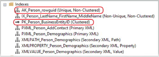
Notice that even though we had a clustered index, (Primary Key Person_BusinessEntityID), SQL used the unique nonclustered index "AK_Person_rowguid" for the count function. And now, the eighth wonder of the world, "what index does the COUNT function use" is finally put to rest.

Using COUNT with GROUP BY

Another way to use the COUNT() function is to add a GROUP BY clause to break down the counts by specified groups. This will return a set of results with a unique count for each group instead of a single count on the whole table.

In the following query, we will count how many times a person whose name starts with "Adr" is listed in the Person.Person table from the AdventureWorks2014 database. We will alias the COUNT column as "TotalRows", use the WHERE clause to filter our results, and of course, we will need to add the GROUP BY clause as well since we are using an aggregate function in our SELECT statement. (You can read more about the GROUP BY clause in the following tutorial: Learning the SQL GROUP BY Clause )

USE AdventureWorks2014;
GO
 
SELECT FirstName, COUNT(*) AS 'TotalRows'
FROM Person.Person
WHERE FirstName LIKE ('Adr%')
GROUP BY FirstName;
GO

Results:

As you can see, this query returns three different counts, one for each first name that starts with "Adr" within the Person.Person table.

Using COUNT with the HAVING Clause

Using the HAVING clause is similar to using the WHERE clause with a COUNT function but with some slight differences. The WHERE clause will not allow a COUNT function directly in-line with that WHERE clause. However, the HAVING clause will allow the COUNT function to reside in-line.

In the sample below, we are counting how many times the Unit Price appears in our table when that Unit Price is listed more than 3,000 times.

USE AdventureWorks2014;
GO

SELECT UnitPrice, COUNT(*) AS 'Total'
FROM Sales.SalesOrderDetail
GROUP BY UnitPrice
HAVING COUNT(UnitPrice) > 3000
ORDER BY UnitPrice DESC;
GO 

Results:

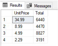
Adding the GROUP BY clause with the HAVING clause retrieves the specific group of a column that matches the condition of the HAVING clause.

SQL COUNT in the WHERE Clause

When adding the COUNT function with a WHERE clause, a first assumption would be to simply add it directly inline like we would with any other filter value. For example, with the HAVING clause as mentioned earlier. On the contrary, T-SQL will not allow an aggregate within the WHERE clause directly.

Using the AdventureWorks2014 sample database, let's count how many times the top three-dollar values are listed in the "Sales.SalesOrderDetail" table. At first glance, you might be thinking of using something like the code below.

USE AdventureWorks2014;
GO

SELECT UnitPrice, COUNT(*) AS myCount
FROM Sales.SalesOrderDetail
WHERE COUNT(UnitPrice) > 3000
GROUP BY UnitPrice;
GO

If so, you will receive the following error:

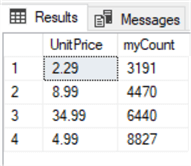
As mentioned before, aggregate functions cannot be placed directly in a WHERE clause unless that WHERE clause is nested inside a subquery or by aliasing the COUNT function. With that said, the code block below demonstrates how you could add the COUNT function in the WHERE clause by using an alias.

USE AdventureWorks2014;
GO
SELECT * FROM
(
   SELECT UnitPrice, Count(*) AS myCount
   FROM Sales.SalesOrderDetail
   GROUP BY UnitPrice
) T 
WHERE myCount > 3000
ORDER BY myCount;
GO

Results:

Filtering the SQL COUNT with the WHERE Clause

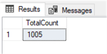
You can filter out specific data by utilizing the WHERE clause in your query. In this query we are counting how many rows contain a name that starts with the letter B in the "FirstName" column of the Person.Person table.

SELECT COUNT(*) AS 'TotalCount'
FROM Person.Person
WHERE firstName LIKE 'B%';
GO

Results:

We can do the same thing by using the CASE statement.

SELECT COUNT(CASE WHEN FirstName LIKE 'B%' THEN 1 END) AS 'TotalCount'
FROM Person.Person;
GO

Results:

Exploring the cost difference between the WHERE clause and CASE.

If we look at the two query plans, we can see they look pretty similar, but the second query scans 19972 rows (the entire table) and the first one scans 1006 rows (only rows that start with "B").  The CASE statement has to be evaluated for each row in the table.

Setting Conditions in COUNT aka COUNTIF

While there is no COUNT(IF) option in T-SQL like you would find in Excel, there is an option to count rows of data only if certain conditions are met. This allows the user to set specific conditions in SQL Server queries that perform in the same manner as the "countif" function in Excel.

Often, we are taught to place either the * (asterisk) or a column name as a parameter within the parenthesis following the COUNT function. However, there are several options to set specific conditions within the COUNT function. An example would be using CASE as in the sample below.

USE AdventureWorks2014;
GO
 
SELECT COUNT(ALL CASE Title 
            WHEN 'Mr.' THEN 1 
            ELSE NULL 
            END) AS 'Total-Mr.'
FROM Person.Person;
GO

Results:

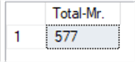
This scenario will work as a filter much like the WHERE clause. Here we are returning the count of rows that only have "Mr." in the Title column, disregarding all other values in that column.

Using DISTINCT in COUNT

Another condition would be to add DISTINCT within the COUNT function parenthesis along with the name of column we wish to "count" the unique values on. Still using the AdventureWorks2014 sample database, let's count how many unique titles that are used in the "Title" column of the Person.Person table, not counting NULL rows.

USE AdventureWorks2014;
GO

SELECT COUNT(DISTINCT Title) AS 'Total Values'
FROM Person.Person;
GO

Results:

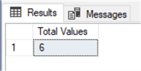
Here we have a count of 6 returned as the amount of distinct titles among all the rows, with the exclusion of any NULL values.

Using COUNT with Partitioning

DBAs often require a count of the result set to be listed in a separate column beside the result set values. This is where the COUNT OVER(PARTITION BY) comes in handy. In the sample below, we are returning the count of orders placed by each customer. Using the COUNT OVER(PARTITION BY) we can "rollup" each customer to get the total number of orders per customer.

In this example, I am filtering our results to only three customers from the Sales.SalesOrderHeader table. However, you can modify the WHERE clause to return the number of orders one particular customer made or remove the WHERE clause to show all of the customer's order quantities.

USE AdventureWorks2014;
GO

SELECT
   SalesOrderNumber,
   CustomerId,
   COUNT(*) OVER (PARTITION BY CustomerId) AS 'Orders for Customer'
FROM Sales.SalesOrderHeader
WHERE CustomerID IN (11254, 11256, 11257);
GO

Results:

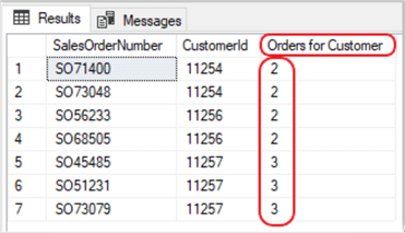
Don't forget, you can also modify the WHERE clause to return a list of your TOP(x) customers by quantity of orders, in case you want to send them a special gift.

Using COUNT_BIG

The COUNT_BIG operates like the COUNT function. The only difference is the data types of the returned values. The COUNT_BIG returns a value with a data type of BIGINT while the COUNT function returns a value with the data type of INT.

A common misconception is that the COUNT function will not work on a column that has a data type of BIGINT. On the contrary, the COUNT function will return a count if the returned count is less than the max value of an INT (2,147,483,647). Otherwise, you will receive the following error and will need to use the COUNT_BIG function.

Msg 8115, Level 16, State 2, Line 4
Arithmetic overflow error converting expression to data type int.

Inversely, you can use the COUNT_BIG function on an INT data type column.

The code block below compares the use of COUNT and COUNT_BIG on an INT data type column from the AdventureWorks2014 sample database.

USE AdventureWorks2014;
GO

SELECT Title, COUNT(*) AS 'Title Count'  
FROM Person.Person
GROUP BY Title;  
GO  

SELECT Title, COUNT_BIG(*) AS 'Title Count'
FROM Person.Person
GROUP BY Title;  
GO  

Results:

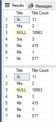
Execution plans compared for the code block above.

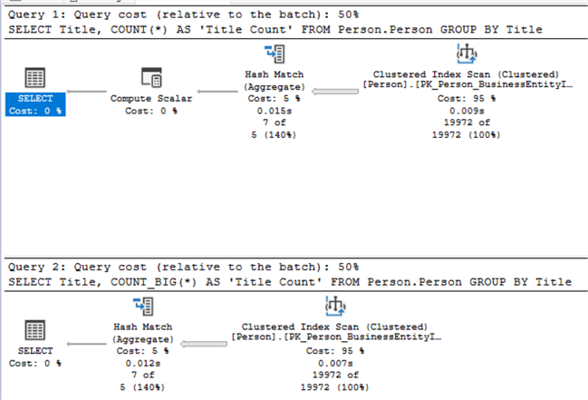
Other than the "Compute Scalar Cost", which has a zero value, the only variance is a couple of milliseconds in time during the "Clustered Index Scan" and the "Hash Match". Consequently, both the COUNT and COUNT_BIG functions are virtually the same in operation and performance.

Counting Rows in Large Tables (105,592,038)

In this section, I decided to go outside the box and not use the standard AdventureWorks2014 sample database. I have included the source code for my sample database at the end of this tutorial (in the Additional Resources section) if you want to follow along. Otherwise, you can simply view the stats that I received during this test.

Working with tables that have a few hundred or even a few thousand rows of data is not a real time-consuming task when doing a count of the rows. But what if your table has a few million or a few billion rows of data. In my test sample table, I have 105,592,038 rows of data in five columns. It's small in comparison to most "big data" environments today, but it should suffice for our testing in this tutorial.

SET STATISTICS TIME ON/OFF – This option will display the CPU time and the "elapsed time" in milliseconds within your "Messages" tab when the query has finished running.

OPTION (MAXDOP 1) – Configures the max degree of parallelism. This option controls how many CPU cores that will be used in the query process. When querying very large tables, you may want to consider using this option. Below is a short list of available options for MAXDOP.

0 – Uses the actual number of available CPU's depending on the current system workload and configuration. This is the default and recommended setting.

1 – Suppresses parallel plan generation. In other words, the operation/query will be executed serially.

2-64 – Limits the number of processes to the specified value. If the provided value is larger than the number of available CPU's listed, then the actual number of CPU's are used.

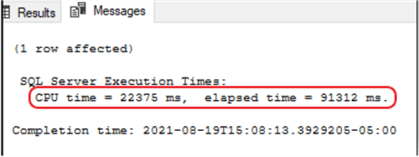
As you can see from the images below, when I first built the table (without any indexes) and populated it with 105+ million rows of data, the time lapse for my count function was 9,132 milliseconds (91.32 seconds).

No index example

USE SampleDataLarge;
GO
 
SET STATISTICS TIME ON;

SELECT COUNT(*)
FROM Sales.Customers
OPTION (MAXDOP 1);

SET STATISTICS TIME OFF;

Results:

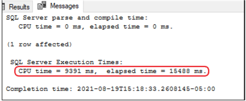
Afterwards, I created a clustered index on one of the smaller columns to improve performance. This simple effort dropped my seek time from 91 seconds to 15.

Clustered index example

USE SampleDataLarge;
GO
 
CREATE INDEX NCCI ON Sales.Customers(CustomerName);
 
SET STATISTICS TIME ON;

SELECT COUNT(*)
FROM Sales.Customers
OPTION (MAXDOP 1);

SET STATISTICS TIME OFF;

Results:

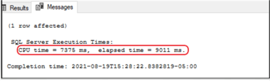
Taking it a step further, I dropped the clustered index and created a nonclustered index. This option dropped my seek time from 15 seconds to 9 seconds.

Nonclustered index example

USE SampleDataLarge;
GO
 
CREATE NONCLUSTERED INDEX NCCI ON Sales.Customers(CustomerName);
 
SET STATISTICS TIME ON;

SELECT COUNT(*)
FROM Sales.Customers
OPTION (MAXDOP 1);

SET STATISTICS TIME OFF;

Results:

In an effort to shrink the seek time to a minimum amount, I made the nonclustered index a "nonclustered columnstore" index.

The columnstore index is only available for SQL Server 2016 (13.x) and later. For older versions of SQL Server, the best performance you will achieve is with the nonclustered index since columnstore is not supported.

With the columnstore index in place, I dropped my scan time to 1.8 seconds. Quiet an improvement over the original 91 seconds. Remember, when dealing with large data amounts, you will need use COUNT_BIG instead of COUNT to return a count value that is more than 2,147,483,647, which is the limit of an INT data type. In our sample, we only had 105+ million rows so the COUNT() function worked just fine.

COLUMNSTORE index example

USE SampleDataLarge;
GO
 
CREATE NONCLUSTERED COLUMNSTORE INDEX NCCI ON Sales.Customers(CustomerName);
 
SET STATISTICS TIME ON;

SELECT COUNT(*)
FROM Sales.Customers
OPTION (MAXDOP 1);

SET STATISTICS TIME OFF;

Results:

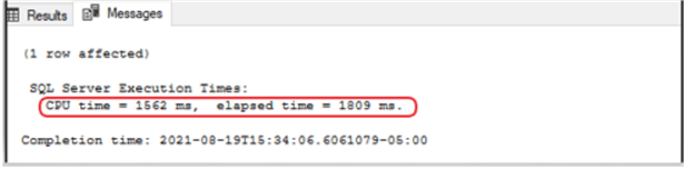
All-in-all, while using the columnstore index, we were able to reduce our scan time by 89 seconds on 105+ million rows. This will be quiet a time saver when your table has a few billion rows of data.

@@ROWCOUNT and @@ROWCOUNT_BIG

These are system function that provide the number of rows affected by a query.

As a best practice it's a good idea to use the @@ROWCOUNT statement when doing an UPDATE or DELETE on a table if you want to know what the row count should be. If the row count results do not match your expected outcome, the transaction should be rolled back. If the number of rows to be affected is more than 2,147,483,647, then you will need to use @@ROWCOUNT_BIG.

There are several options when using the @@ROWCOUNT function, you could simply return the number of rows affected by an insert, delete, etc. in a SELECT statement by calling the PRINT function.

In the following code block, we are attempting to update a row that doesn't exist. Normally we would expect a result of "x number of rows affected" but since the row doesn't exist, the PRINT @@ROWCOUNT will return a zero.

USE AdventureWorks2014;
GO

UPDATE HumanResources.Employee
SET JobTitle = 'Exec'
WHERE NationalIDNumber = 123456789

PRINT @@ROWCOUNT;
GO

Often, you will want to return a statement if the condition was met and a different statement if the condition was not met. Providing the fact that we know how many rows we are updating, in this scenario it is one row, we can set an IF – ELSE statement to return one of two possible comments when the job is complete.

USE AdventureWorks2014;
GO

UPDATE HumanResources.Employee
SET JobTitle = 'Exec'
WHERE NationalIDNumber = 123456789

IF @@ROWCOUNT = 1
   PRINT 'Rows were updated'
ELSE 
   PRINT 'Warning: No rows were updated.' ;

GO

Results:

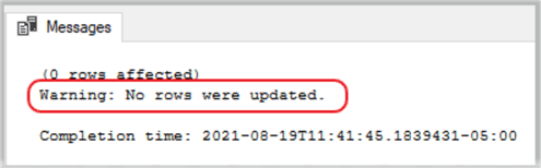
Again, since the row didn't exist, no rows were affected and SSMS printed out the statement contained in the ELSE condition.

Play around with these options and change the condition operator from (=) to (!=) or (>), etc. to see the results.

How to work with NULLs and how NULLs impact the COUNT function

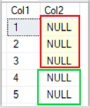
I think the first order of business for this section would be to understand what NULL is and what it is not. In terms of a relational database, a NULL value indicates an unknown value. That's not to say it's a zero, because a zero is a set value. A NULL is more of an "empty placeholder" waiting for a value to be assigned. There is a noticeable difference between a NULL value and the text "NULL".

In SQL Server Management Studio (SSMS) the visual distinction for an observer is the yellow highlighting in the cell containing a NULL when a table is queried. The image below shows the yellow highlighting in column 2 (Col2) for rows one through three. Rows four and five do not have the yellow highlighting because they contain an actual value, in this case it's the word "NULL".

You can insert NULL into a table by using something like the code below.

INSERT INTO Table1 VALUES (NULL),(NULL),(NULL); 

Notice there are no quote marks around the words NULL in the statement. This creates a NULL or "empty placeholder" for that tuple. However, the following command will insert a text value in those columns, and the tuples will no longer be NULL.

INSERT INTO Table1 VALUES ('NULL'),('NULL'),('NULL'); 

Now that we understand what NULL is and what it is not, let's move on to working with NULL in a table by counting NULL values and then excluding NULL values during a COUNT function.

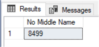
Using the AdventureWorks2014 sample database, we want to count how many people do not have a middle name listed in the Person.Person table.

SELECT COUNT(*) AS 'No Middle Name'
FROM Person.Person
WHERE MiddleName IS NULL;
GO

Results:

On the flip side, let's now count how many people do have a middle name listed in the Person.Person table.

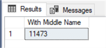
SELECT COUNT(*) AS 'With Middle Name'
FROM Person.Person
WHERE MiddleName IS NOT NULL;
GO

Results:

This works fine if you use the COUNT(*) function, but what if you specify the column name in the COUNT function instead of using the asterisk? Using the same query as listed above, we will replace the asterisk with the column name and see that it returns zero for the count.

SELECT COUNT(MiddleName) AS 'No Middle Name'
FROM Person.Person
WHERE MiddleName IS NULL;
GO

Results:

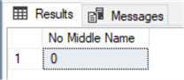
This is happening because the function ignores all the NULL values.

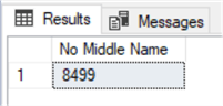
 In order to count the NULL values, you will first need to convert them to different values and then apply the aggregate function. The sample code below shows an easy fix for this scenario.

SELECT COUNT(ISNULL(MiddleName,0)) AS 'No Middle Name'
FROM Person.Person
WHERE MiddleName IS NULL;
GO

Results:

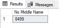
As an alternative, you could get the same results as above by using the * (asterisk) inside the COUNT parenthesis like in the sample below.

SELECT COUNT(*) AS 'No Middle Name'
FROM Person.Person
WHERE MiddleName IS NULL;
GO

Results:

Unless you need to specifically use an aggregate in the SELECT statement, it's a best practice to keep your code as simple as possible.

Using COUNT with OFFSET FETCH

The OFFSET and FETCH clauses are options directly associated with the ORDER BY clause. They allow you to limit the number of rows to be returned by a query. However, you cannot have an OFFSET-FETCH without an ORDER BY clause. Consequently, when we run the following samples, the results are going to look different than the previous SQL commands we have been executing in the first part of this tutorial.

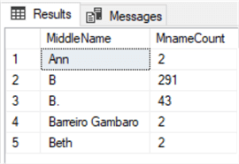
First, let's take a snapshot of the first eight rows of the middle name only with and without NULL values for the middle name.

SELECT TOP(8) 
    MiddleName
   ,COUNT(MiddleName) AS 'MnameCount'
FROM Person.Person
WHERE MiddleName IS NULL OR MiddleName IS NOT NULL
GROUP BY MiddleName
ORDER BY MiddleName;
GO

Results:

The top three rows, highlighted in the red box above, will be the top three that will be removed during an OFFSET-FETCH statement as shown below.

SELECT 
    MiddleName
   ,COUNT(MiddleName) AS 'MnameCount'
FROM Person.Person
WHERE MiddleName IS NULL OR MiddleName IS NOT NULL
GROUP BY MiddleName
ORDER BY MiddleName
OFFSET 3 ROWS FETCH NEXT 5 ROWS ONLY;
GO

Results:

As a result, our OFFSET-FETCH is working as expected by offsetting (omitting), the top three rows regardless if the "middlename" is populated with data or contains a NULL.

Using COUNT with XML

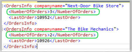
The SQL query below, uses the aggregate COUNT() function, as well as the aggregate MAX() function, to return XML data (information) about the orders for each customer in a temporary table named "CustomerOrders".

In this example we have two companies. The first company, "Next-Door Bike Store" shows three orders while the company "The Bike Mechanics" shows only two orders. The SELECT statement uses a XQuery FLWOR expression to step through the orders. The COUNT() function, shown as "COUNT($i/Order)", returns a total for each company.

DECLARE @x AS XML;
SET @x='
<CustomersOrders>
 
<Customer custid="292" companyname="Next-Door Bike Store">
<Order orderid="10692" orderdate="2007-10-03" />
<Order orderid="10702" orderdate="2007-10-13" />
<Order orderid="10952" orderdate="2008-03-16" />
</Customer>
 
<Customer custid="298" companyname="The Bike Mechanics">
<Order orderid="10308" orderdate="2006-09-18" />
<Order orderid="10926" orderdate="2008-03-04" />
</Customer>
 
</CustomersOrders>';
 
SELECT @x.query('
for $i in //Customer
return
<OrdersInfo>
{ $i/@companyname }
 
<NumberOfOrders>
{ count($i/Order) }
</NumberOfOrders>
 
<LastOrder>
{ max($i/Order/@orderid) }
</LastOrder>
 
</OrdersInfo>
');

Results

The XQuery FLWOR expression formats the XML returned by the SELECT statement of the query. FLWOR is an acronym for "For, Let, Where, Order by and Return". A FLWOR expression is in essence, a foreach loop. You can use FLWOR expressions to iterate through any sequence. You can learn more about FLWOR from Microsoft's Docs by clicking this link: FLWOR Statement and Iteration

Summary

There is a lot you can do with the COUNT function. It doesn't always have be called as just COUNT(*) or COUNT(columnName). As you can see in the samples above, we can also add expressions inside the COUNT parenthesis, add a GROUP BY or HAVING clause and so much more.

Next Steps

• Take these a step further by modifying the code and experimenting \ learning.
• Test some of those scenarios to see if you can expand on their functionality.
• Review the following tips and other resources:
  • COUNT(Transact-SQL)
  • SQL Server COUNT() Function Performance Comparison
  • Basic SQL Server XML Querying
  • SQL Server Row Count for all Tables in a Database

Additional Resources

Creating a large data table for use with the section "Counting Rows in Large Tables" from above. The following code block will create a database table that we will populate with 105,592,038 rows of data and will require approximately 56GB of space on your hard drive.

-- Test table
USE SampleDataLarge;
GO
CREATE SCHEMA Sales AUTHORIZATION dbo;
GO
CREATE TABLE Sales.Customers (
   CustomerID BIGINT NOT NULL
   , CustomerName CHAR(100) NOT NULL
   , CustomerAddress CHAR(100) NOT NULL
   , Comments CHAR(189) NOT NULL
   , LastOrderDate DATE
   );
GO

Warning: running the following code block will take several hours for completion, depending on your computer's performance. For example: on my personal computer with an i7 3.8 GHz 4 core processer, 32GB of RAM and a Crucial MX500 2TB hard drive, it took about 10 hours to complete.

-- Test data
DECLARE @rdate DATE
DECLARE @startLoopID BIGINT = 1
DECLARE @endLoopID BIGINT = 105592038 -- Amount of Rows you want to add
DECLARE @i BIGINT = 1
WHILE (@i <= 105592038) -- Make sure this is the same as the "@endLoopId" from above
WHILE @startLoopID <= @endLoopID
BEGIN
    SET @rdate = DATEADD(DAY, ABS(CHECKSUM(NEWID()) % 10950 ), '1970-01-01'); -- The "10950" represents 30 years, the date provided is the starting date.
    SET @startLoopID = @startLoopID + 1;
 
    INSERT INTO Sales.Customers(CustomerID, CustomerName, CustomerAddress, Comments, LastOrderDate)
   VALUES 
   (
      @i,
      'CustomerName' + CAST(@i AS CHAR),
      'CustomerAddress' + CAST(@i AS CHAR),
      'Comments - Lorem ipsum dolor sit amet, consectetur adipiscing elit' + CAST(@i AS CHAR),
      (@rdate)
   )
   SET @i += 1;
END

About the author

Aubrey Love is a self-taught DBA with more than six years of experience designing, creating, and monitoring SQL Server databases as a DBA/Business Intelligence Specialist. Certificates include MCSA, A+, Linux+, and Google Map Tools with 40+ years in the computer industry. Aubrey first started working on PC’s when they were introduced to the public in the late 70's.

This author pledges the content of this article is based on professional experience and not AI generated.

View all my tips