Problem
With the rise of cloud, automation and managed services, the role of the Database Administrator has pivoted towards Data Engineering. The focus is to maintain, secure, and cleanse data in order for data analysis and decision making by the business.
How can we start using modern data analysis tools with our current SQL Server infrastructure? Further, how can we start providing end users and decision makers with important insights about our data, without spending extra money on enterprise data analysis tools?
Solution
Using programming languages like Python, and free libraries like scikit-learn for machine learning, we can provide valuable machine learning insights with our existing data. Couple this with a modern driver like mssql-python, we can securely access our data, while outperforming old drivers like pyodbc which requires ODBC.
Environment Setup
Connecting and analyzing data is pretty straightforward.
Use the following infrastructure to get started:
- SQL Server instance with the AdventureWorks2022 database (we will use a local container for this tip).
- Latest version of Python, you can download and install from here. In my case, I am using a Mac, so after downloading the .pkg file you have to follow the setup instructions, which is very similar for Windows.

Once done, you can close the wizard.

Use Mssql-python for Python connectivity to SQL Server:
- Open-source and developed by Microsoft, this driver is optimized for SQL Server and Azure family of databases.
- It provides better performance than the usual pyodbc connector, and supports many new features.
- To install, run the following commands
- brew install openssl
- Install the mssql driver:
- pip install mssql-python
Scikit-learn Python library for our data analysis:
- Run the following to install
- pip install -U scikit-learn
Install additional Python libraries for presentation and data handling (pandas, NumPy and matplotlib):
- Run the following to install
- pip install pandas numpy matplotlib
Once you install Python and the required libraries, we are ready to start analyzing our data.
Example 1: Learn the Basics with K-Means clustering
One simple analysis with the Machine Learning (ML) library scikit-learn, is K-means clustering. This will automatically group similar behaving items together. This analysis will help us understand the basics of an ML implementation on Python. We will try to cluster together Products based on sales performance.
First, we create a query to determine the products by Total Quantity and by Total Revenue.
SELECT
    p.ProductID,
    p.Name AS ProductName,
    SUM(d.OrderQty) AS TotalQty,
    SUM(d.LineTotal) AS TotalRevenue
FROM Sales.SalesOrderDetail d
JOIN Production.Product p
    ON d.ProductID = p.ProductID
GROUP BY p.ProductID, p.Name;
Sample execution:

Basic Python code:
import mssql_python
import pandas as pd
from sklearn.cluster import KMeans
import matplotlib.pyplot as plt
import matplotlib.ticker as mtick

# 1. Load product data from SQL

connection_string = (
    "SERVER=tcp:localhost,1433;"
    "DATABASE=AdventureWorks2022;"
    "UID=<yourUser>;"
    "PWD=<yourPWD>;"
    "Encrypt=no;"
)

conn = mssql_python.connect(connection_string)

query = """
SELECT
    p.ProductID,
    p.Name AS ProductName,
    SUM(d.OrderQty) AS TotalQty,
    SUM(d.LineTotal) AS TotalRevenue
FROM Sales.SalesOrderDetail d
JOIN Production.Product p
    ON d.ProductID = p.ProductID
GROUP BY p.ProductID, p.Name;
"""
df = pd.read_sql(query, conn)
conn.close()


# 2. K-Means clustering

X = df[["TotalQty", "TotalRevenue"]]

kmeans = KMeans(n_clusters=3, random_state=1)
df["Cluster"] = kmeans.fit_predict(X)

# 3. Plot clusters

plt.figure(figsize=(8, 6))
scatter = plt.scatter(
    df["TotalQty"],
    df["TotalRevenue"],
    c=df["Cluster"],
    cmap="viridis",
    s=80,
    alpha=0.8
)

# Axis labels
plt.xlabel("Total Quantity Sold (Units)")
plt.ylabel("Total Revenue (USD)")

# Axis formatting
ax = plt.gca()
ax.xaxis.set_major_formatter(mtick.StrMethodFormatter("{x:,.0f}"))
ax.yaxis.set_major_formatter(mtick.StrMethodFormatter("${x:,.0f}"))

plt.title("Product Segmentation Using K-Means Clustering")
plt.grid(alpha=0.3)


plt.tight_layout()
plt.show()
Explaining every section
- Load product data from SQL
- We connect to the AdventureWorks2022 database and run the select query we created earlier. We load that result into a Pandas DataFrame so Python can work with it.
- K-Means clustering
- Using kmeans function, we will divide products on three features (n_clusters) so we can have high, medium and low performing sections. We will use amount and quantity as our input features for the model. Then using fit_predict, we get the automatic classification.
- Plot clusters
- The last section, is just the generation of the chart for the results using pyplot. We generate a scatter chart that shows the amount vs quantity, and each point represents a product. Using an alpha of 0.3 we divide each cluster category on a different color. This is just a visual formatting option, and at last, we present the chart.
If we run the script above, we will get a chart like this:

We can see that we successfully categorized each product into high, medium and low performing products.
For simplicity of the demo, we did not label each product, nor added a hover animation, because that will increase the code complexity.
But with something as simple as that, you can present to business the top performing products and begin to make decisions.
Now that we have learned the basics, we will perform more complex analysis.
Example 2: Demand Forecasting to Predict Next Month’s Product Sales
We will create a model to forecast the next month of sales for products based on previous month’s sales.
First, we create our view to get the sales by month for products:
CREATE OR ALTER VIEW dbo.MonthlyProductSales AS
SELECT
    d.ProductID,
    p.Name AS ProductName,
    CAST(DATEFROMPARTS(YEAR(h.OrderDate), MONTH(h.OrderDate), 1) AS date) AS MonthStart,
    SUM(d.OrderQty) AS TotalQty
FROM Sales.SalesOrderDetail AS d
INNER JOIN Sales.SalesOrderHeader AS h
    ON d.SalesOrderID = h.SalesOrderID
INNER JOIN Production.Product AS p
    ON d.ProductID = p.ProductID
GROUP BY
    d.ProductID,
    p.Name,
    DATEFROMPARTS(YEAR(h.OrderDate), MONTH(h.OrderDate), 1);
GO

SELECT * FROM dbo.MonthlyProductSales;
Sample data:

Now using the following script, we will predict the future sales, and for demonstration, we will display the first product on the list:
import mssql_python
import pandas as pd
from sklearn.ensemble import RandomForestRegressor
from sklearn.metrics import mean_absolute_error, r2_score
import matplotlib.pyplot as plt

# Load monthly product sales from SQL
connection_string = (
    "SERVER=tcp:localhost,1433;"
    "DATABASE=AdventureWorks2022;"
    "UID=<youruser>;"
    "PWD=<YourPassword>;"
    "Encrypt=no;"
)

conn = mssql_python.connect(connection_string)

query = "SELECT ProductID, ProductName, MonthStart, TotalQty FROM dbo.MonthlyProductSales;"
df = pd.read_sql(query, conn)
conn.close()

df["MonthStart"] = pd.to_datetime(df["MonthStart"])
df = df.sort_values(["ProductID", "MonthStart"])

# Create time-series features per product

def make_supervised(group, n_lags=3):
    g = group.copy()

    # Lags: previous months' quantities
    for lag in range(1, n_lags + 1):
        g[f"lag_{lag}"] = g["TotalQty"].shift(lag)

    # Simple rolling average of last 3 months (as of previous month)
    g["rolling_mean_3"] = g["TotalQty"].rolling(window=3).mean().shift(1)

    # Month of year for simple seasonality signal
    g["month"] = g["MonthStart"].dt.month

    # Target: next month's quantity
    g["target_next"] = g["TotalQty"].shift(-1)

    return g

df_feat = (
    df.groupby("ProductID", group_keys=False)
      .apply(make_supervised)
)

# Drop rows where any feature / target is missing (lags, rolling, next month)
df_feat = df_feat.dropna(subset=["lag_1", "lag_2", "lag_3",
                                 "rolling_mean_3", "month", "target_next"])

feature_cols = ["lag_1", "lag_2", "lag_3", "rolling_mean_3", "month"]
X = df_feat[feature_cols]
y = df_feat["target_next"]

#Train/test split by time

cutoff_date = df_feat["MonthStart"].quantile(0.8)

train_mask = df_feat["MonthStart"] < cutoff_date
test_mask = ~train_mask

X_train, X_test = X[train_mask], X[test_mask]
y_train, y_test = y[train_mask], y[test_mask]

# Train model

model = RandomForestRegressor(
    n_estimators=300,
    random_state=1,
    n_jobs=-1
)

model.fit(X_train, y_train)

# Evaluate

y_pred = model.predict(X_test)
mae = mean_absolute_error(y_test, y_pred)
r2 = r2_score(y_test, y_pred)

print(f"MAE (units) = {mae:,.1f}")
print(f"R²          = {r2:,.3f}")

# Choose one product to demonstrate, you can modify the code to select another product
counts = df.groupby("ProductID")["MonthStart"].count()
product_to_plot = counts.sort_values(ascending=False).index[0]

# Get product name for display
product_name = (
    df.loc[df["ProductID"] == product_to_plot, "ProductName"]
      .iloc[0]
)

print(f"Product selected for demo: {product_to_plot} - {product_name}")

hist = (
    df[df["ProductID"] == product_to_plot]
    .sort_values("MonthStart")
    .reset_index(drop=True)
)

# Build the SAME features for that product
hist["lag_1"] = hist["TotalQty"].shift(1)
hist["lag_2"] = hist["TotalQty"].shift(2)
hist["lag_3"] = hist["TotalQty"].shift(3)
hist["rolling_mean_3"] = hist["TotalQty"].rolling(3).mean().shift(1)
hist["month"] = hist["MonthStart"].dt.month

hist_feat = hist.dropna(subset=["lag_1", "lag_2", "lag_3", "rolling_mean_3", "month"])

last_row = hist_feat.iloc[[-1]]
X_future = last_row[feature_cols]

# Predict next month units for this product
future_qty = model.predict(X_future)[0]

# Compute next month date
last_month = last_row["MonthStart"].iloc[0]
next_month = (last_month + pd.offsets.MonthBegin(1))

print(f"Last month in data: {last_month.date()}, units={int(last_row['TotalQty'].iloc[0])}")
print(f"Forecast next month: {next_month.date()}, units≈{future_qty:.1f}")

# Chart: history + next-month forecast for one product

plt.figure(figsize=(10, 6))

# Historical actuals
plt.plot(hist["MonthStart"], hist["TotalQty"], marker="o", label="Actual monthly sales")

# Forecast point
plt.scatter(next_month, future_qty, color="red", marker="x", s=80, label="Forecast next month")
plt.plot([hist["MonthStart"].iloc[-1], next_month],
         [hist["TotalQty"].iloc[-1], future_qty],
         "--", color="red", alpha=0.7)

plt.xlabel("Month")
plt.ylabel("Units sold")
plt.title(f"{product_name} - Monthly Sales and Next-Month Forecast")
plt.legend()
plt.grid(alpha=0.3)
plt.tight_layout()
plt.show()
Code explanation:
- Load monthly product sales from SQL
- In this section, we connect to SQL Server using our mssql-python driver and get the view we previously created, then load the view into a dataframe.
- Create time-series features per product
- For each (ProductID, MonthStart) row, we want to know what happened the last 3 months, and then add a placeholder for the next month prediction. We update a dataframe, and then for this demo, we delete nulls or products without data.
- Train/test split by time
- We will use the first 80% of the months for training the model, and 20% for testing.
- Train Model
- Using RandomForestRegressor to generate decision trees, each tree learns its own way to map features, so in our case, predict future months.
- The forest’s prediction is the average of all trees. We use 300 trees for this demo, but you can adjust, if needed. More trees means more accurate prediction, but also more computing work, that can increase the model evaluation on large datasets.
- Evaluate
- With the test data we separate on step 3, we evaluate the accuracy of the model vs the real values. For that we get Median Absolute Error which represents how far or close we calculated from the actual values. For our demo, we were off by 1,000 units. And the R2 that measures the accuracy of our model with 1 being perfect accuracy and the accuracy decreases as we get far from 1, there is no “good” or “bad” value, but in finance, anything close to 0.5 is acceptable. If you need more precision, you can increase number of trees or increase the raining data.
- Forecast
- Now that we are happy with our training model, we can start forecasting for future months. For that we pick one product. For our demo we will choose the first one on the list, but you can change the code to do it for all products or select it on runtime. We get the information for previous months for that product, we remove nulls if they exist. Then using the previous trained model, we evaluate the information to predict next month, and then print the forecasted value.
- Generate Forecast Chart
- Our last step is to generate a chart to show previous months and forecast for the product we selected. Since this is a demo, we will just chart one, as charting multiple products can be really convoluted and hard to read. We use a simple scatter chart for the points, and then join the points with lines, then we add the forecasted value as a red point, with a dashed line.
If we run the script above, we will get a chart like this:

Corresponding values:
- MAE (units) = 44.3
- R² = 0.489
- Product selected for demo: 707 – Sport-100 Helmet, Red
- Last month in data: 2014-06-01, units=77
- Forecast next month: 2014-07-01, units≈295.3
The R2 value is pretty close to what we wanted to achieve, and the MAE indicate that we will have an approximate variation of 45 units.
This analysis gives the business enough insight on how to prepare the product stock for future months.
Example 3: Customer Segmentation
We will segment our customers using K-means, but this time using multiple features: Total Spend, Avg Order Value, Number of Orders and Days Since Last Purchase. This segmentation will be automatic, and we will have to interpret it until we have the results, for this demo we will segment into 4 categories.
First, we build our query to get the required information by each client:
CREATE OR ALTER VIEW dbo.CustomerBehaviorFeatures AS
WITH OrderAgg AS (
    SELECT
        h.CustomerID,
        COUNT(DISTINCT h.SalesOrderID)         AS NumOrders,
        SUM(h.SubTotal)                        AS TotalSpend,
        AVG(h.SubTotal)                        AS AvgOrderValue,
        MIN(h.OrderDate)                       AS first_order_date,
        MAX(h.OrderDate)                       AS last_order_date
    FROM Sales.SalesOrderHeader AS h
    GROUP BY h.CustomerID
)
SELECT
    o.CustomerID,
    o.TotalSpend,
    o.AvgOrderValue,
    o.NumOrders,
    DATEDIFF(DAY, o.last_order_date, MAX(o.last_order_date) OVER ()) AS DaysSinceLastPurchase
FROM OrderAgg   AS o
GO

SELECT * FROM dbo.CustomerBehaviorFeatures;
This will return the required data:

Then we perform the analysis with this script:
import mssql_python
import pandas as pd
from sklearn.preprocessing import StandardScaler
from sklearn.cluster import KMeans
import matplotlib.pyplot as plt
import matplotlib.ticker as mtick


# 1. Load customer info from SQL

connection_string = (
    "SERVER=tcp:localhost,1433;"
    "DATABASE=AdventureWorks2022;"
    "UID=<youruser>;"
    "PWD=<YourPassword>;"
    "Encrypt=no;"
)

conn = mssql_python.connect(connection_string)

query = "SELECT * FROM dbo.CustomerBehaviorFeatures;"
df = pd.read_sql(query, conn)
conn.close()

# Drop rows with missing values
df = df.dropna()

# 2. Build feature matrix for clustering

feature_cols = [
    "TotalSpend",
    "AvgOrderValue",
    "NumOrders",
    "DaysSinceLastPurchase"
]

X = df[feature_cols].copy()

# Scale features so dollars, counts and days are on similar ranges
scaler = StandardScaler()
X_scaled = scaler.fit_transform(X)

# 3. K-Means customer segmentation

kmeans = KMeans(n_clusters=4, random_state=1)
df["Cluster"] = kmeans.fit_predict(X_scaled)

currency_fmt = mtick.StrMethodFormatter("${x:,.0f}")

# 4. Chart 1: AOV vs Order Frequency
plt.figure(figsize=(9, 6))
plt.scatter(
    df["AvgOrderValue"],
    df["NumOrders"],
    c=df["Cluster"],
    cmap="plasma",
    alpha=0.8,
)

plt.gca().xaxis.set_major_formatter(currency_fmt)
plt.xlabel("Average Order Value (USD)")
plt.ylabel("Number of Orders per Customer")
plt.title("Customer Segmentation - AOV vs Order Frequency")
plt.grid(alpha=0.3)
plt.show()

# 5. Chart 2: Total Spend vs Last Purchase

plt.figure(figsize=(9, 6))
plt.scatter(
    df["TotalSpend"],
    df["DaysSinceLastPurchase"],
    c=df["Cluster"],
    cmap="plasma",
    alpha=0.8,
)

plt.gca().xaxis.set_major_formatter(currency_fmt)
plt.xlabel("Total Spend (USD)")
plt.ylabel("Days Since Last Purchase")
plt.title("Customer Segmentation - Total Spend vs last Purchase")
plt.grid(alpha=0.3)
plt.show()- Load customer information from SQL Server
- Similar to the previous examples, we get the previous query and load into a pandas dataframe so we can manipulate it.
- Build feature matrix for clustering
- We select the features we want to analyze for clustering. We normalize them using feature scaling, so amounts and days have similar scale.
- K-Means clustering
- Using kmeans function, we will divide products on four features (n_clusters) so we can have multiple customer classifications. Then using fit_predict, we get the automatic classification.
- Plot chart 1 AOV vs Order Frequency
- Since we do not know how we will intrepretate each cluster, we will generate 2 charts to have better insights, since we are clustering using 2 features and we can only plot 2. This first one, we will plot average of order vs order frequency.
- Plot chart 2: Total Spend vs Last Purchase
- To have a proper context when reading the results, we will generate a second chart, this time we will plot the total spend vs last purchase by customer. With the help of the 2 charts, we will be able to have a better understanding of the clustering.
If we run the script above, we will generate 2 charts like this:
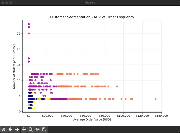

We can see the following with the help of the 2 charts:
- The pink dots as our most important customers, as they spend the most in the shortest timeframe, make those customers happy so they can keep buying.
- The blue dots are the less spending customers.
- The yellow dots represent one-time customers, those who rarely buy us.
- Finally, the purple dots are frequent customers, but they spend little money, so probably you should focus to improve customer relationships on this category, with better deals or price discounts.
Next Steps
- You can explore more sci-kit demos here.
- You can learn how to deploy local SQL environments from VSCode here.
- Learn more about new MSSQL Python driver here.

Eduardo Pivaral is an MCSA, SQL Server Database Administrator and Developer with over 15 years of experience working in large environments.
- MSSQLTips Awards: Trendsetter (25+ tips) – 2020 | Author of the Year Contender – 2019 | Rookie of the Year – 2018


