Problem
While PowerPivot isn’t necessarily “new technology” I think businesses are trying to move towards it because Excel savvy end users can create their own reports without tying up IT resources. KPI’s are just another addition to PowerPivot that allows users to visually analyze data across millions of rows.
In a previous tip I explained how to use PowerPivot with Excel 2013. This tip will focus on creating calculated fields and KPI’s in PowerPivot. Check it out.
Solution
A KPI (Key Performance Indicator) is a graphical representation that displays progress against a predefined measure or business goal. KPIs make it easier for end users to evaluate the amount of progress without reading a bunch of data.
If you are new to PowerPivot, try looking over some of these tips first to gain a foundation on what PowerPivot is and some of the basics of creating dashboards.
In this example, I’ll use AdventureWorksDW2012 sample data so you can follow along with me.
Let’s get started.
Enabling PowerPivot in Excel 2013
To enable PowerPivot, open Excel, go to File, Options, Add-Ins, select COM Add-ins and click Go. This will open up the COM Add-Ins dialog box. Click “Microsoft Office PowerPivot for Excel 2013” and hit OK. After successfully enabling PowerPivot, the tab should appear at the top of the Excel spreadsheet:
Importing Data
Open Excel, click the PowerPivot tab, Manage:

Upon clicking Manage, a new window should appear. From this window, you will import data. Click From Database and select From SQL Server:

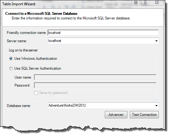
Type in the Server Name, Authentication mode, and browse to the AdventureWorksDW2012 database:
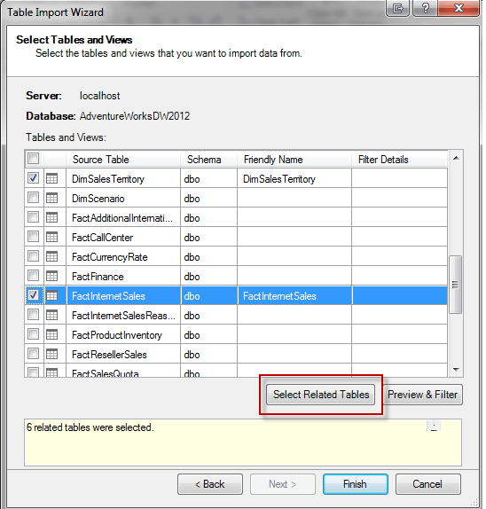
Click Next, choose “Select from a list of tables and views to choose the data to import” and click Next. The next screen is where we will select our data to import. For this example, choose FactInternetSales and click “Select Related Tables”. The Select Related Tables button enables you to automatically select every table that is related to the source table selected:
After clicking Finish, the import will begin. Once the import finishes successfully you should be able to view all the tables separated into sheets:

Creating PivotTable
Before creating a KPI we will need to slice and dice our data into a PivotTable. To do this, click PivotTable on the ribbon bar and choose New Worksheet:

Our boss wants a PowerPivot report that displays quarterly profit percentages on AdventureWorks’ total sales. Before we design the report we need to determine the calculation that we’ll need to get to this point. If I take the product cost and subtract it from the sales cost I’ll get my total profit in dollars. Then I’ll take that amount and divide it by the total product cost, which will give me the total percentage.
OK, easy enough. Let’s design the dashboard.
First, we need to slice the dashboard up into quarters since we only want to report on quarterly numbers. To do this, drilldown the DimDate header and drag down CalendarYear and CalendarQuarter into the Rows section: (Make sure CalendarYear is on top of CalendarQuarter)

We now have a PivotTable with something on it. Next we need to add some values. Drilldown the FactInternetSales header and drag SalesAmount down to the Values section:
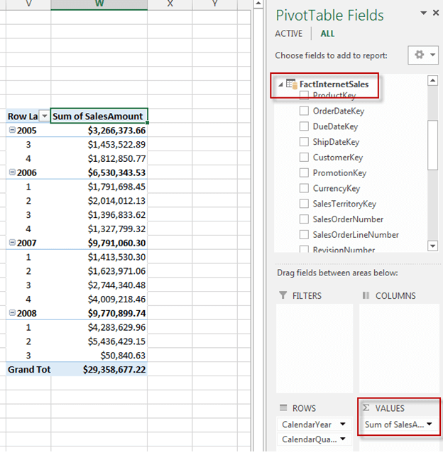
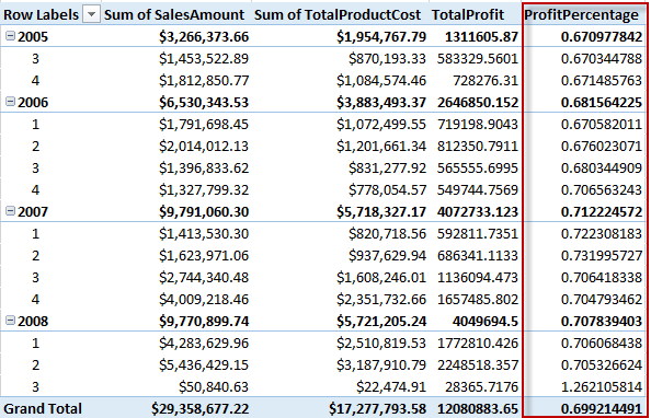
Our Pivot table is coming along. We now have the total sales amount broken down by each quarter. Next we’ll need to add the total product cost. Drag TotalProductCost to the Values section below SalesAmount:

Create Calculated Fields
So far, so good. The next column we need to add will be a calculated column. We will need to determine the profit from each quarter. To determine the profit we will need to subtract the sales amount from the product cost.
Under the PowerPivot tab, click Calculated Fields and select New Calculated Field:

On the Calculated Field window select the table name, give the field a name, and enter your formula. For our example, we will use the FactInternetSales table, name it TotalProfit, and enter our formula as =SUM(FactInternetSales[SalesAmount])-SUM(FactInternetSales[TotalProductCost])

We have now created a calculated field that will subtract the sales amount from the product cost. After clicking OK, the new column should appear to the right:

Now we need to create a calculated field that will give us the percentage of profit. To do this, we will need the outcome of the above calculated field.
Choose New Calculated Field and enter the following:
- Table name: FactInternetSales
- Calculated field name: ProfitPercentage
- Formula: =[TotalProfit]/SUM(FactInternetSales[TotalProductCost])
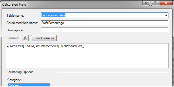
In this example we used the outcome of TotalProfit and divided it by the Total Product Cost. After clicking OK, the new column should appear to the right:
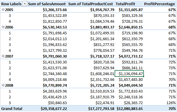
To format the calculated columns, highlight the column and right click and choose Format Cells:
Create KPI
The dashboard is almost is complete except for the KPI. To add a KPI click KPI’s, New KPI:

On the KPI screen we will need to choose the calculated field that we are basing our KPI values on. We will also choose absolute value because we didn’t create another calculated value to compare with. We will change the Absolute Value to 1 and move the thresholds like below. The status thresholds are reporting on the percentage in decimal form, for example, 70% looks like .70.

After clicking OK, we notice that the KPI’s have been added to the right:

Next Steps
- To find out more about KPI’s in PowerPivot, click here to visit Microsoft’s Office site.
- Creating basic PowerPivot dashboards are fairly easy and usually don’t require any IT resources except to provide a data model and possibly security access to the database for importing data.
- You can find other tips regarding Microsoft Excel Integration here.

Brady has been in the IT industry for 10+ years. He has worked in administrative roles using MSSQL 2000 to 2012 as well as Sharepoint 2007 and 2010. He currently serves as a Database Administrator in Nashville, TN. You can view his blog @ http://www.sqlbrady.com.
- MSSQLTips Awards: Trendsetter (25+ tips) – 2013