By: Andrea Gnemmi | Comments | Related: > SQL Server vs Oracle vs PostgreSQL Comparison
Problem
This is the fourth tutorial in the series about different behaviors of basic SQL statements in SQL Server, Oracle and PostgreSQL. This time we dive a little bit into more advanced features like window functions (also called windowing or in Oracle analytic functions) which obviously are different between the three RDBMS systems...or are they?
Solution
Window functions are very useful in SELECT queries mainly for extractions, reports and generally data warehouse oriented tasks. We will take a look at the different syntaxes and possibilities, but also at the similarities of these operations in the SQL Server, Oracle and PostgreSQL as well as some performance optimization tips.
SQL Window Functions
First of all, let’s take a look at the definition of what we call window functions in standard SQL. Window functions are aggregates based on a set of rows, similar to an aggregate function like a GROUP BY, but in this case this aggregation of rows moves or slides across a number of rows so we have a sort of sliding window or window frame, thus the name window functions.
It is best explained using examples, so let’s start with the basic concepts of partitioning the data set, this need arises mostly for reporting purposes, but also for paging and in various context not limited to a data warehouse.
The basic syntax for all three RDBMS uses the OVER (PARTITION BY…) clause, so let’s walk through some examples.
I will use the github freely downloadable database sample Chinook, as it is available in multiple RDBMS formats at this link. It is a simulation of a digital media store, with some sample data, all you have to do is download the version you need and you have all the scripts for data structure and data inserts.
SQL Window Functions Example 1
First we will do a simple example where we group data by music genre and show the percentage of sales for each item over the entire result set.
SQL Server
Suppose that we need to create a small report returning the sales importance by genre in percentage, this is a typical example where a windowing function is best and simplest:
select
   distinct genre.[Name],
   cast(SUM(Quantity) OVER (PARTITION BY genre.name)as decimal(10,5)) / SUM(Quantity) OVER () * 100 AS Perc
from InvoiceLine
inner join Track on InvoiceLine.TrackId=Track.TrackId
inner join Genre on Track.GenreId=Genre.GenreId
order by Perc desc
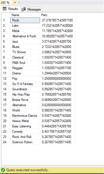
Note that I had to CAST the quantity value to a decimal from an integer otherwise I would have got just 0 as a result, because there were no decimals. I have used the OVER(PARTITION BY…) clause partitioning data by genre and in this way I obtained the SUM aggregation by genre and immediately divided it by the total obtained without partitioning the data, all in one query!
Oracle
Let’s see the syntax in Oracle now:
select
   distinct genre.name,
   SUM(Quantity) OVER (PARTITION BY genre.name) / SUM(Quantity) OVER () * 100 AS Perc
from chinook.InvoiceLine
inner join chinook.Track on InvoiceLine.TrackId=Track.TrackId
inner join chinook.Genre on Track.GenreId=Genre.GenreId
order by Perc desc;
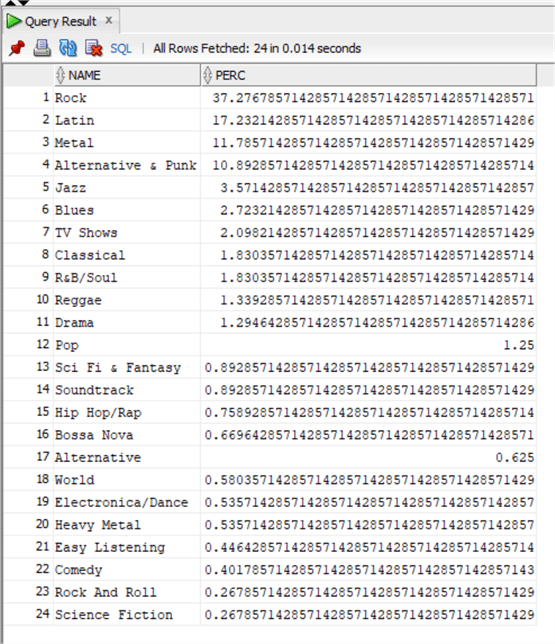
As you can see we have exactly the same syntax and we do not even need to do the CAST trick in order to have the correct result.
PostgreSQL
Finally the same example with PostgreSQL:
select
   distinct "Genre"."Name",
   cast(SUM("Quantity") OVER (PARTITION BY "Genre"."Name") /cast(SUM("Quantity") OVER () as decimal (8,3))*100 as decimal (5,3)) as Perc
from "InvoiceLine"
inner join "Track" on "InvoiceLine"."TrackId"="Track"."TrackId"
inner join "Genre" on "Track"."GenreId"="Genre"."GenreId"
order by Perc desc;
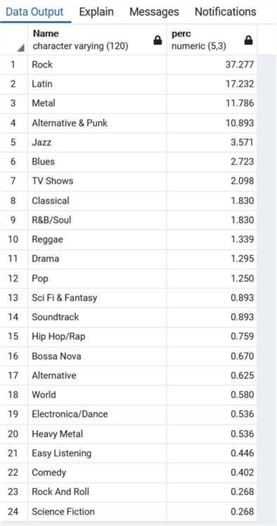
Again here like in SQL Server we need to CAST at least one of the integer values as decimal in order to obtain the correct result, in this case just for final visualizations I casted the final operation.
In summary, the syntax for the OVER clause is the same in all three RDBMS. In this case I have used an aggregate function together with the window function, but there are also other operators.
SQL Window Functions Example 2
Let’s make another classic example in which the windowing functions come to the rescue, we suppose that we need to obtain the average time passed between one purchase (first row) and the next (following rows) for each customer.
SQL Server
;WITH InvCust AS
   (SELECT
       DISTINCT CustomerID, InvoiceDate AS cur_d
      ,next_d = LEAD(InvoiceDate, 1) OVER (PARTITION BY CustomerID ORDER BY InvoiceDate)
    FROM Invoice)
,customer_avg as
   (SELECT
       CustomerID,cur_d,next_d
      ,dif_day  = DATEDIFF(DAY, cur_d, next_d),avg_cust = AVG(DATEDIFF(DAY, cur_d, next_d)) OVER (PARTITION BY CustomerID)
      ,avg_all  = AVG(DATEDIFF(DAY, cur_d, next_d)) OVER ()
    FROM InvCust)
select distinct
   customer.customerid,
   FirstName + ' ' + lastname as Customer,
   country,avg_cust,
   avg_all
from customer_avg
inner join customer on Customer.CustomerId=customer_avg.CustomerId
order by avg_cust
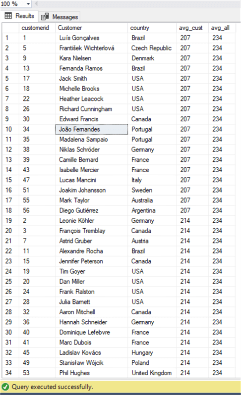
As you can see with this query, the first CTE is used with the LEAD function for the previous InvoiceDate as we have partitioned the data set by CustomerID and ordered it by InvoiceDate.
Then with the second CTE we have taken this data and calculated the average days by customer and average in total using a simple DATEDIFF on the partitioned by CustomerID window. We have also obtained the average for all orders by using the OVER clause, in this way we do not have a partition, or better the partition is the whole table like in the previous example.
Finally, we add data such as customer name and country to complete our extraction and we order it in the last query. Nice!
We have made use in this case of one of the analytic functions together with the OVER (PARTITION BY …) that’s to say LEAD, which accesses a row given an offset (in our case 1 which is also the default), so that we are able to compare the value of the current row with the following row.
Oracle
WITH InvCust AS
   (SELECT DISTINCT CustomerID, InvoiceDate AS cur_d, LEAD(InvoiceDate, 1) OVER (PARTITION BY CustomerID ORDER BY InvoiceDate) as next_d
    FROM chinook.Invoice)
,customer_avg as
   (SELECT CustomerID,cur_d,next_d
      ,(next_d-cur_d)as dif_day, AVG((next_d-cur_d)) OVER (PARTITION BY CustomerID) as  avg_cust
      ,AVG(next_d-cur_d) OVER () as avg_all
    FROM InvCust)
select distinct customer.customerid,FirstName||' '||lastname as Customer, country,cast(avg_cust as decimal(5,2)) as avg_customer, cast(avg_all as decimal(5,2)) as avg_allcust
from customer_avg
inner join chinook.customer
on Customer.CustomerId=customer_avg.CustomerId
order by avg_customer, customerid;
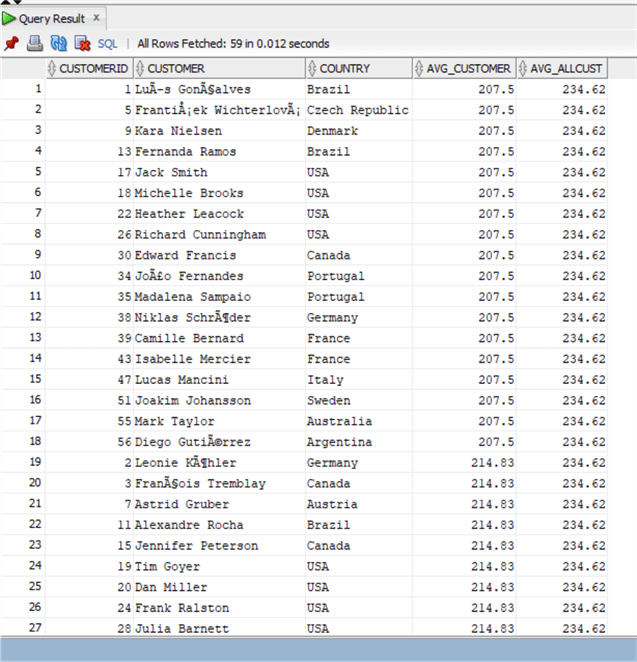
Also in this case the syntax of the OVER (PARTITION BY…) and LEAD functions are the same, what changes are the syntax for date operations that can be performed directly with a - and some other minor cosmetic features that I added in order to visually have the same result.
PostgreSQL
WITH InvCust AS
   (SELECT DISTINCT "CustomerId", "InvoiceDate" AS cur_d, LEAD("InvoiceDate", 1) OVER (PARTITION BY "CustomerId" ORDER BY "InvoiceDate") as next_d
    FROM "Invoice")
,customer_avg as
   (SELECT "CustomerId",cur_d,next_d
      ,next_d-cur_d as dif_day,AVG(next_d-cur_d) OVER (PARTITION BY "CustomerId") as avg_cust
      ,AVG(next_d-cur_d) OVER () as avg_all
    FROM InvCust)
select distinct "Customer"."CustomerId","FirstName"||' '||"LastName" as Customer, "Country",avg_cust, avg_all
from customer_avg
inner join "Customer"
on "Customer"."CustomerId"=customer_avg."CustomerId"
order by avg_cust;
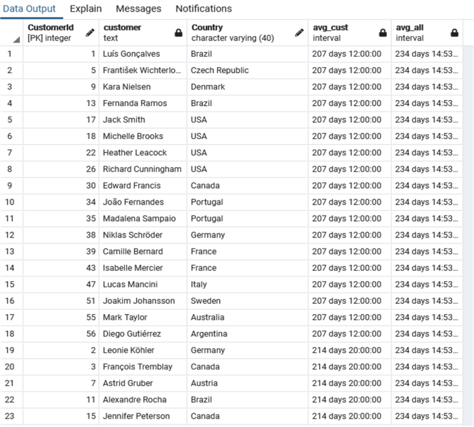
For this example, apart from the usual syntax differences on date operations, the window function works with the same behavior.
SQL Window Functions Example 3
We have seen examples with an analytic function and an aggregate function. We can also use ranking functions that can be used inside a window function, let’s see an example.
Let’s imagine that we need to obtain the rank of our customers based on their total invoices:
SQL Server
;with customer_invoice as
   (select
      customerid,
      SUM(Total) as Total_customer
    from Invoice
    group by customerid)
,classification as
   (select customerid,
      rank() over (order by total_customer desc) as classifica,
      dense_rank() over (order by total_customer desc) as classifica_dense,
      Total_customer
    from customer_invoice)
select classification.customerid, Firstname, lastname, Country, Total_customer,classifica, classifica_dense
from classification
inner join Customer on classification.customerid = customer.customerid
order by classifica
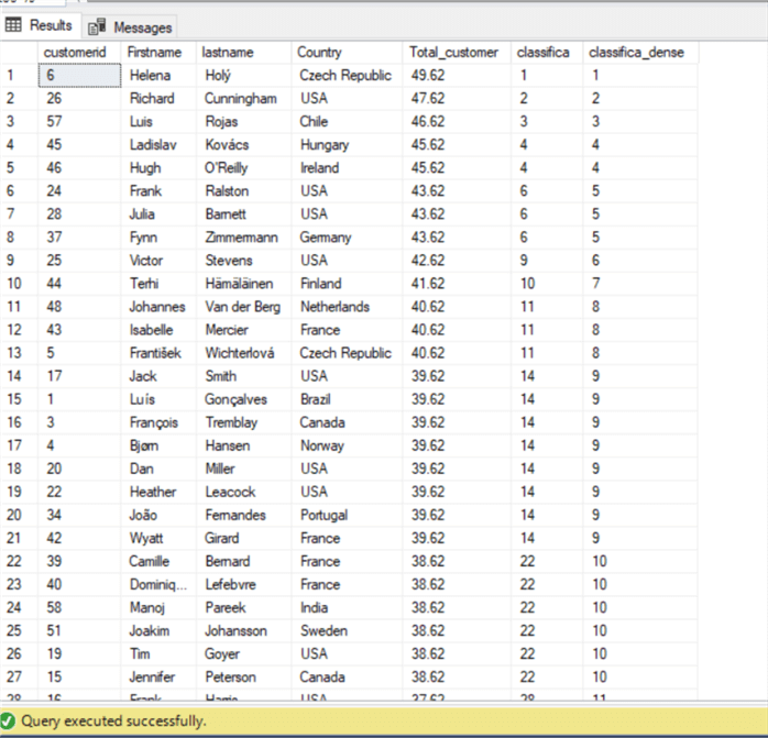
First of all I’ve obtained in a CTE the total invoiced amount by customer with a simple aggregation using GROUP BY. Then I applied the RANK function using the total invoiced amount by customer as the order by (ASC | DESC) in a descending order. In this way I’ve obtained the rank of each customer. I’ve made an example also using the DENSE_RANK function. The difference between the two is that with RANK, ties in ranking repeat and leave gaps with the next value while DENSE_RANK ranking does not leave gaps in rank values as you can see in the example result set above.
Oracle
with customer_invoice as
  (select customerid, SUM(Total) as Total_customer
   from chinook.Invoice
   group by customerid)
,classification as
  (select customerid, rank() over (order by total_customer desc) as classifica,
      dense_rank() over (order by total_customer desc) as classifica_dense,
      Total_customer
   from customer_invoice)
select classification.customerid,  Firstname, lastname, Country, Total_customer,classifica, classifica_dense
from classification
inner join chinook.Customer on classification.customerid = customer.customerid
order by classifica;
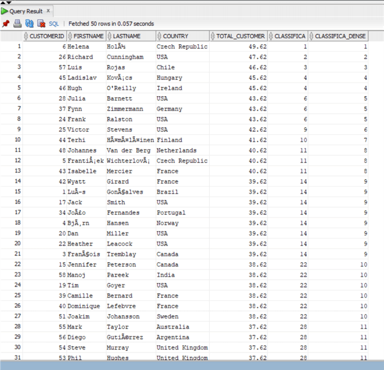
In Oracle we have exactly the same syntax.
PostgreSQL
with customer_invoice as
  (select "CustomerId", SUM("Total") as Total_customer
   from "Invoice"
   group by "CustomerId")
,classification as
  (select "CustomerId", rank() over (order by total_customer desc) as classifica,
      dense_rank() over (order by total_customer desc) as classifica_dense,
      Total_customer
   from customer_invoice)
select classification."CustomerId",  "FirstName", "LastName", "Country", Total_customer,classifica, classifica_dense
from classification
inner join "Customer" on classification."CustomerId"="Customer"."CustomerId"
order by classifica;
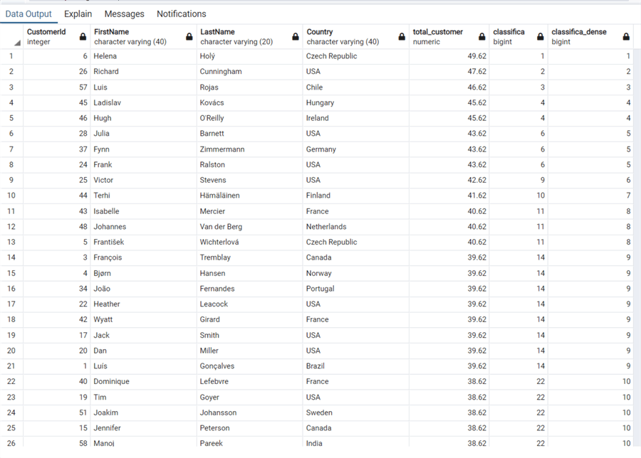
In PostgreSQL we see the same syntax and meanings for the ranking functions.
SQL Window Functions Example 4
Another very interesting use case for window functions are running and moving aggregates. Let’s look at another example in the following query which we’d like to obtain the number of invoices completed every month in 2012 as specified in the WHERE clause. We also want to have the sum of invoices of just the preceding three months and the average, as well as the moving sum in total:
SQL Server
SELECT
   YEAR(invoicedate) AS Year_Invoice,
   MONTH(InvoiceDate) AS Month_Invoice,
   COUNT(*) AS Invoice_Count,
   SUM(COUNT(*)) OVER(ORDER BY YEAR(InvoiceDate), MONTH(InvoiceDate) ROWS BETWEEN 2 PRECEDING AND CURRENT ROW) AS Count_of_3_Month,
   AVG(COUNT(*)) OVER(ORDER BY YEAR(InvoiceDate), MONTH(InvoiceDate) ROWS BETWEEN 2 PRECEDING AND CURRENT ROW) AS Avg_of_3_Month,
   SUM(COUNT(*)) OVER(ORDER BY YEAR(InvoiceDate), MONTH(InvoiceDate)) as Moving_count
FROM Invoice
WHERE InvoiceDate >= '01/01/2012' AND InvoiceDate < '01/01/2013'
GROUP BY YEAR(InvoiceDate), MONTH(InvoiceDate)
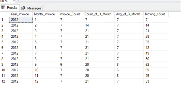
As you can see in this case we are using frames inside the partition in order to obtain running and moving aggregates, by specifying the frame, we can calculate reverse running totals and moving aggregates. In this case the frame is defined by ROWS BETWEEN 2 PRECEDING AND CURRENT ROW so we get the actual row and the two preceding for the count and average of the three months, and we just use the OVER(ORDER BY YEAR,MONTH) to have the running total of invoices.
Oracle
SELECT
   extract(YEAR from invoicedate) AS Year_Invoice,
   extract(MONTH from to_date(InvoiceDate, 'dd/mm/yyyy')) AS Month_Invoice,
   COUNT(*) AS Invoice_Count,
   SUM(COUNT(*)) OVER(ORDER BY extract(YEAR from invoicedate), extract(MONTH from to_date(InvoiceDate, 'dd/mm/yyyy')) ROWS BETWEEN 2 PRECEDING AND CURRENT ROW) AS Count_of_3_Month,
   cast(AVG(COUNT(*)) OVER(ORDER BY extract(YEAR from invoicedate), extract(MONTH from to_date(InvoiceDate, 'dd/mm/yyyy'))ROWS BETWEEN 2 PRECEDING AND CURRENT ROW) as numeric (4,2)) AS Avg_of_3_Month,
   SUM(COUNT(*)) OVER(ORDER BY extract(YEAR from invoicedate), extract(MONTH from to_date(InvoiceDate, 'dd/mm/yyyy'))) as Moving_count
FROM chinook.Invoice
WHERE InvoiceDate >= to_date('01/01/2012','dd/mm/yyyy') AND InvoiceDate < to_date('01/01/2013','dd/mm/yyyy')
GROUP BY extract(YEAR from invoicedate), extract(MONTH from to_date(InvoiceDate, 'dd/mm/yyyy'));
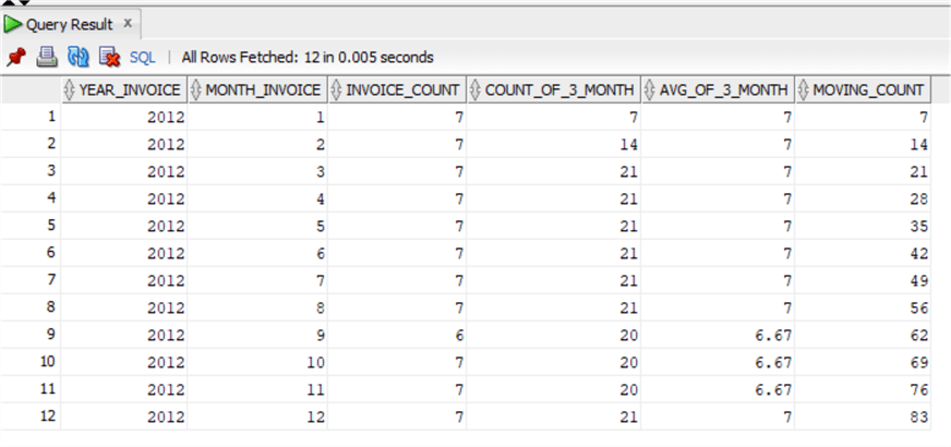
Again except for the date functions, we have exactly the same syntax, note that I had to cast the average as the approximation to the integer was automatically returning 7, so we can see that approximation is done differently between SQL Server and Oracle.
PostgreSQL
SELECT
   extract(YEAR from "InvoiceDate") AS Year_Invoice,
   extract(MONTH from "InvoiceDate") AS Month_Invoice,
   COUNT(*) AS Invoice_Count,
   SUM(COUNT(*)) OVER(ORDER BY extract(YEAR from "InvoiceDate"), extract(MONTH from "InvoiceDate") ROWS BETWEEN 2 PRECEDING AND CURRENT ROW) AS Count_of_3_Month,
   AVG(COUNT(*)) OVER(ORDER BY extract(YEAR from "InvoiceDate"), extract(MONTH from "InvoiceDate")ROWS BETWEEN 2 PRECEDING AND CURRENT ROW) AS Avg_of_3_Month,
   SUM(COUNT(*)) OVER(ORDER BY extract(YEAR from "InvoiceDate"), extract(MONTH from "InvoiceDate")) as Moving_count
FROM "Invoice"
WHERE "InvoiceDate" >= to_date('01/01/2012','dd/mm/yyyy') AND "InvoiceDate" < to_date('01/01/2013','dd/mm/yyyy')
GROUP BY extract(YEAR from "InvoiceDate"), extract(MONTH from "InvoiceDate");
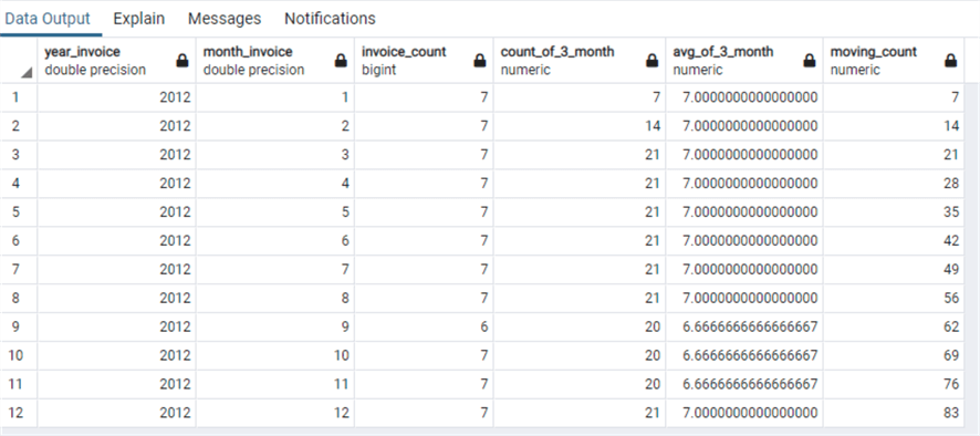
And also with PostgreSQL we have the same syntax and result, again the only difference is the date functions.
Tuning SQL Window Functions
We have seen the usefulness of the window functions in the previous examples, but it is very important to note that some precautions must be taken in order to have good performance with these queries.
First of all we have seen that they are super useful together with CTEs, but CTEs in SQL Server are not always the best in terms of performance and sometimes temp tables are better, especially if we also need to apply an index (more on that), see this blog post What’s Better, CTEs or Temp Tables?
But is this true also on the other two RDBMS? The short answer is no.
In Oracle we do not even have the concept of a temporary table like SQL Server and in PostgreSQL we have Global temporary tables which are permanent database objects that store data on disk and visible to all sessions. Here is a link with a nice explanation of this concept and examples: Oracle Global Temporary Table.
So an alternative of CTEs in Oracle are subqueries, which perform quite well, even better than CTEs sometimes, but it is very hard to read them and also it is difficult to do recursive queries, that is where in my opinion CTEs are best used as they can be referred to between the different parts of the query as we have seen in the examples.
In PostgreSQL, CTEs generally perform better than a temporary table, so it is not normally advisable to use one, unless you need to create an index on it. The explanation on why a temporary table is slower than a CTE in PostgreSQL is that a temp table generates VACUUM work on the system catalogs that a CTE doesn't, so it needs an extra round trip to create and fill it and it requires extra work in the server's cache management.
BUT, in PostgreSQL there is another caveat about CTEs, in versions previous to 12, PostgreSQL will always materialize a CTE. That can be very bad for performances as a query that should touch a small amount of data instead reads a whole table and possibly spills it to a tempfile. This behavior, that is completely different from the other RDBMS, as I wrote before this has been modified and corrected from version 12 of PostgreSQL. A nice blog post about this problem is this: PostgreSQL’s CTEs are optimisation fences.
Back to the concern of window function performance, the most common bottleneck and the easiest to check and correct is the sort operator, that’s to say the PARTITION BY and the ORDER BY parts of the OVER clause. In this case it is possible to add an index on the columns used in the PARTITION BY and in the ORDER BY, then performances will greatly improve and we will have a more efficient query. This is true in all three RDBMS and a nice explanation with examples in SQL Server is in this article SQL Server Window Functions Performance Improvement.
Next Steps
- We have seen that all three RDBMS have the same syntax and basically the same functionally, finally something standard in all RDBMS!
- I really recommend reading the documentation of window functions as there are a complete list of all available functions as well as loads of examples:
- Further tips regarding window functions:
About the author
 Andrea Gnemmi is a Database and Data Warehouse professional with almost 20 years of experience, having started his career in Database Administration with SQL Server 2000.
This author pledges the content of this article is based on professional experience and not AI generated.
View all my tips


