Working with Columns and Properties in PowerPivot for Excel

By: Dattatrey Sindol | Comments (7) | Related: > Microsoft Excel Integration

Problem

I want to know if it is possible to show or hide columns in PowerPivot Tables and if it is possible to apply custom sorting on columns like sorting data in ColumnA based on data in ColumnB similar to SSAS functionality. Also, I would like to know, what are the other common properties which can be set at the column level.

Solution

In this tip we will take a look at the following properties of columns in a table in PowerPivot for Excel:

Description
Data Type
Format
Visibility
Sorting

Pre-requisites

To start working with column properties using the steps in this tip, you need to first go through the following tips in the same sequence and setup your Excel/PowerPivot workbook using the steps outlined in these tips.

Setting Column Descriptions

By default, the name of the column acts/shows up as its description in front-end/reporting tools like Excel. Description is a very useful feature and can be used to provide additional information about a column to the end users, while they are working with the data in tools like Excel.

Follow the below listed steps to set a description for any of the columns in a table. For this demonstration, we will set the description for "FullDateAlternateKey" column in "DimDate" table.

Go to "DimDate" table.
Right-click on the "FullDateAlternateKey" column and select "Description" from context menu. This will open the "Column Description" dialog box.
In the "Column Description" dialog box enter the description as "Fully Qualified Date" as shown below.

This is the description which the end users will see in column tooltips while analyzing/working with this data in tools like Excel.

Setting Column Data Types

When the data is pulled from the underlying data source into PowerPivot, the data type of columns is automatically detected and applied to the columns by PowerPivot. In the below screenshot, we can see that the data type of the "FullDateAlternateKey" column in "DimDate" table is set to "Date". Since the data present in this column is of date data type, we can leave it as is.

Data Type of FullDateAlternateKey column

If we want to change the data type of any of the columns in PowerPivot, the following list of data types are supported:

Currency
Date
Decimal Number
Whole Number
Text
TRUE/FALSE (Boolean)

One should be careful while changing the data type of a column, as it might lead to loss of precision or data in certain scenarios. In many scenarios, you might just want to change the data format (like Date only instead of Date Time as discussed in the next section).

Formatting Column Data

Data in columns can be formatted by applying specific formatting styles and is very important from a reporting standpoint. Let's see how formatting can be applied to columns.

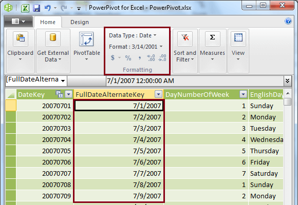
Go to "DimDate" table and select "FullDateAlternateKey" column and notice in the "Formatting" section of the Home tab of the Top Ribbon that, the "Data Type" is set to "Date" and "Format" is set to "*3/14/2001 1:30:55 PM" as shown below. Since this column is of type "Date", we will leave the "Data Type" as is.
Change the "Format" to "3/14/2001" since this column contains only dates and hence the time part is set to "12:00:00 AM" as shown above. The column Format and the data in the column after applying this formatting looks as shown below.
Now go to the "FactResellerSales" table and select "SalesAmount" column. Notice the properties set on this column as shown below.
Depending upon the underlying column's data type, PowerPivot applies some formatting on the column by default. In this particular scenario, the following formatting exists on the "SalesAmount" column by default.
- Data Type: This property is used to indicate the type of data present in the column. This property is set to "Currency" for the "SalesAmount" column, since the underlying column's data type is set to "Money" at the time of importing the data into PowerPivot.
- Format: This property is used to set the "Format" on the column's data like "General", "Decimal Number", "Whole Number", "Currency", "Percentage", and "Scientific" depending upon the type of data present in the column. Not all format options are available for all types of data in each column. The Format property for "SalesAmount" columns is set to "Currency". This is again due to the data type of the underlying column at the time of data import.
- Apply Currency Format: This property is used to set/apply specific currency symbols for the column. This property is set to "$ English (United States)" for the "SalesAmount" column. Depending upon the country/currency, this property can be set accordingly.
- Apply Percentage Format: This property can be used for those columns which contain percentage data. This property is not set on this column since the data is not a percentage.
- Thousands Separator: This property is used to apply commas in numeric data. This is similar to formatting available in other office tools like Excel. This property has been set on the "SalesAmount" column.
- Increase Decimal: This button is used to increase the number of digits that can appear in the data after the Decimal Point.
- Decrease Decimal: This button is used to decrease the number of digits that can appear in the data after the Decimal Point. Click on "Decrease Decimal" button twice and reduces the number of decimal places to "Zero", so that the data in the column looks as shown below.
  
  Do the same thing for "TaxAmt" and "Freight" columns as shown above.

Controlling Column Visibility

Columns of a table can be either visible or hidden from the client tools. This is useful especially for reporting users, as some of the columns may not be required for analysis. For instance, an English User analyzing the data, would not require the Spanish Name of the product. Similarly some of the columns which are not required for analysis can be hidden from the client tools.

Hiding columns can be done in two different ways/views: in Diagram View and in Grid View

Hiding Column(s) in Diagram View

To demonstrate this, let's hide the "SpanishCountryRegionName" in "DimGeography" table. To hide a column from Client Tools, follow the below listed steps.

Go to Diagram View by clicking on "Diagram View" in the Top Ribbon or by clicking on the "Diagram View" button in the bottom right corner of the PowerPivot window.
Right Click on the "SpanishCountryRegionName" column in "DimGeography" table which needs to be hidden from the Client Tools and select "Hide from Client Tools" from the context menu as shown below.
The columns which are hidden from the client tools appear dim or lighter in color in the diagram view as shown below.

Hiding Column(s) in Grid View

To demonstrate this, let's hide the "FrenchCountryRegionName" in "DimGeography" table. To hide a column from Client Tools, follow the below listed steps.

Go to Grid View by clicking on "Grid View" in the Top Ribbon or by clicking on the "Grid View" button in the bottom right corner of the PowerPivot window.
Right Click on the "FrenchCountryRegionName" column in "DimGeography" table which needs to be hidden from the Client Tools and select "Hide from Client Tools" from the context menu as shown below.
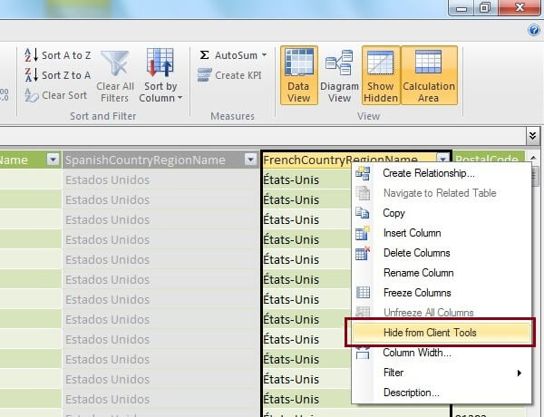
The columns which are hidden from client tools appear grayed out in color in the grid view as shown below.

Always hide those columns from the Client Tools which are not required during analysis. This will greatly help the reporting users and will reduce confusion.

Applying Custom Sorting on Column Data

By default the columns are sorted based on the data type of the columns and the same sorting order is used to display the data in the reports (Pivot Charts/Tables). Data in the tables can be sorted based on specific columns in "Ascending" or "Descending" order based on the Data Type of the data present in the column. However, in some scenarios, we might want to a sort a column based on another column such as the end users wish to see the Month as "January", "February", etc... but they want to sort based on the Month Number and not Alphabetically. This is when custom sorting comes into the picture. Let's see how the data in one column can be sorted based on the data present in another column.

To demonstrate this, let's sort the Month Names in DimDate dimension based on Month Number. Add a new column as "SortedMonth" (This is to ensure we have both the original column and the sorted column) using the following steps:

Click on the second cell in the "Add Column" field in DimDate table in PowerPivot windows (at the extreme right)
Enter the formula: "=[Month]" and hit enter.
Right click on the column and select "Rename Column" from the context menu and rename it to "SortedMonth".
With the Column Selected, go to the Home Tab on the Top Ribbon and click on "Sort by Column" as shown below.
This will bring up the "Sort by Column" dialog box. Ensure that "Sort Column" drop down is set to "SortedMonth" and set the "By Column" to "MonthNumber".

As we can see, from the above demonstrations, there are various properties associated with columns in PowerPivot for Excel.

Next Steps

Try the above options and properties on columns in PowerPivot tables.
Check out my previous tips

About the author

Dattatrey Sindol has 8+ years of experience working with SQL Server BI, Power BI, Microsoft Azure, Azure HDInsight and more.

This author pledges the content of this article is based on professional experience and not AI generated.

View all my tips