Problem
The debate over star schemas and snowflake schemas has been around in the dimensional modeling for a while. Designers with a transactional database design background cannot resist creating normalized dimension tables even though they agree to use the star schema. Data redundancy and duplication in dimension tables does not make them comfortable and they argue that normalized dimension tables require less disk space and are easier to maintain. To make them use star schemas consistently, we need to explain what normal forms should be used in the data warehouse design, why we should use them and how to design a dimensional model.
Solution
Kimball recommended star schemas in his book [1]. He stated that ease-of-use and higher query performance delivered by the star schema outweighed the storage efficiencies provided by the snowflake schema. His other book [2] indicated fact tables were typically normalized to the third normal form (3NF) and dimension tables are in the second normal form (2NF), or possibly in third normal form (3NF).
This solution is organized as follows: First, we review Kimball’s opinions in the support of the star schema. Second, we review some basic database concepts. Then, we compare the normalization and denormalization. In the end, we introduce two design processes to create a dimensional model. All of these conclude that flattened denormalized dimension tables should be used in the dimensional modeling.
Resist Habitual Normalization Urges
Kimball advocated the star schema and provided six reasons in his book [1];
(1) The business users and their BI applications prefer easy data access through a simple data structure;
(2) Most query optimizers understand the structure of star schemas;
(3) Fact tables take up more disk space compared to the dimension tables. The disk space savings by using snowflake schemas are not significant;
(4) A star schema enhances the users’ ability to browse within a dimension and understand the relationship between dimension attribute values;
(5) A snowflake schema needs numerous tables and joins, therefore increases the query complexities and slows query performance;
(6) A snowflake schema prohibits the use of bitmap indexes, which are advantageous to index low-cardinality columns;
In general, dimension tables typically are highly denormalized with flattened many-to-one relationships within a single dimension table. Kimball also mentioned that a snowflake schema is permissible under certain circumstances. I have a different opinion. Any snowflake dimension tables will have a potentially negative impact on ease-of-use and query performance.
Relational Database Basics Review
To avoid ambiguity, let’s review some fundamental terms of database design [3] that are used in both entity-relationship modeling and dimensional modeling.
What is a Database?
Burns [4] quoted some definitions for databases in his book. A typical definition is that a database is an organized collection of logical data. When we move into the world of relational databases, a database is made up of relations, each representing some type of entity. A tuple represents one instance of that entity and all tuples in a relation must be distinct. An attribute is a characteristic of an entity. The logical terms “relation”, “tuple” and “attribute” correspond to physical terms “table”, “row” and “column”, respectively.
A relation schema consists of the name of a relation followed by a list of its attributes. A database schema, which is composed of many relation schemas and connections between relations, represents the logical view of a database. An attribute domain that is the type of values for the attribute should consist of atomic values, which indicates multivalued or divisible attributes are not acceptable.
Keys and Constraints
A super-key is a subset of attributes in a relation that are always unique. A key is a minimal super-key. No attribute can be removed from the key to maintain the uniqueness. If a relation has more than one key, each is called a candidate key. A prime attribute is an attribute that belongs to some candidate keys. A nonprime attribute is an attribute that does not belong to any candidate key.
The primary key is a candidate key whose values are used to uniquely identify tuples in a relation. A primary key can consist of one attribute or multiple attributes.
Normalization
Redundancy occurs when more than one tuple in a relation represent the same information. Redundancy creates update anomalies.
Assuming X and Y are two sets of attributes in a relation, a functional dependency (FD) is a constraint between X and Y. When only X can determine Y (X -> Y), X is the determinant and Y is the dependent attribute(s).
When the determinant is a subset of the primary key, the functional dependency is a partial dependency. On the other side, when the determinant is not part of the primary key, the functional dependency is a transitive dependency. If the primary key is a single attribute, there is not a partial dependency in the relation.
Decomposing a schema is a technique to break up the tables into more tables to eliminate redundancy and simplify enforcing of functional dependency.
Database normalization is the process of analyzing given relation schemas based on their functional dependencies and primary keys to minimize redundancy and update anomalies.
A relation is in 1NF if and only if the domain of each attribute contains only atomic values, and the value of each attribute contains only a single value from that domain [5]. A relation is in 2NF if it is in 1NF and all partial dependencies are removed. When all transitive dependencies are removed from the relation in 2NF, the relation is normalized to 3NF.
Denormalization
Denormalization is the process of transforming higher normal forms to lower normal forms via storing the join of higher normal form relations as a base relation. Denormalization increases the performance in data retrieval at cost of bringing update anomalies to a database.
Introduction to Data Normalization
Informally, a relational database relation is often described as "normalized" if it meets 3NF [6]. We use data collected in an invoice [7] from Acme Industries, a fictitious company, to go through the normalization process. This is a simplified example used to explain normalization and is not enough for a real-world application.
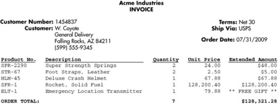
Figure 1 – Invoice Example
We represented partial information from the invoice in the tabular form, shown in Table 1. Given the information, the primary key of this relation consists of multiple attributes: “Customer Number”, “Order Date”, “Terms” and “Ship Via”. A tuple in this relation represents one invoice.
| Customer Number | Customer City | Customer State | Order Date | Terms | Ship Via | Product Number | Quantity | Unit Price | Extended Amount |
| 1454837 | Falling Rocks | AZ | 2009-07-31 | Net 30 | USPS | SPR-2290 STR-67 HLM-45 SFR-1 ELT-1 | 2 2 1 1 1 | 24.00 2.50 67.88 128200.40 79.88 | 48.00 5.00 67.88 128200.40 0 |
Table 1 – INVOICE
First Normal Form (1NF)
The un-normalized relation, shown in table 1, has multiple-valued attributes, for example, the product number cell contains multiple products. To convert this relation to 1NF, we expend the key so that multiple values in one cell become separate tuples in the original relation. The Table 2 presents the data in 1NF:
| Customer Number | Customer City | Customer State | Order Date | Terms | Ship Via | Product Number | Quantity | Unit Price | Extended Amount |
| 1454837 | Falling Rocks | AZ | 2009-07-31 | Net 30 | USPS | SPR-2290 | 2 | 24.00 | 48.00 |
| 1454837 | Falling Rocks | AZ | 2009-07-31 | Net 30 | USPS | STR-67 | 2 | 2.50 | 5.00 |
| 1454837 | Falling Rocks | AZ | 2009-07-31 | Net 30 | USPS | HLM-45 | 1 | 67.88 | 67.88 |
| 1454837 | Falling Rocks | AZ | 2009-07-31 | Net 30 | USPS | SFR-1 | 1 | 128200.40 | 128200.40 |
| 1454837 | Falling Rocks | AZ | 2009-07-31 | Net 30 | USPS | ELT-1 | 1 | 79.88 | 0 |
Table 2 – INVOICE LINE ITEM
The attribute “Product Number” was added to the primary key and the primary key of the relation now contains the attributes: “Customer Number, Order Date, Terms, Ship Via and Product Number”. It is observed that the level of detail in Table 2 has changed to a line item in an invoice.
Second Normal Form (2NF)
To convert 1NF to 2NF, we need to remove partial dependencies where the determinant is a subset of the primary key. We always consider the determinant and dependant to be sets of attributes even though they may have a single attribute. When removing partial dependencies, we usually start with the smallest determinant. If each determinant has the same number of attributes, we pick a dependency with the smallest dependant. We use the following steps to obtain 2NF relations:
First, let us find all partial dependencies. The attribute “Product Number” determines the attributes “Unit Price.” The attribute “Customer Number” determines the attributes “Customers City” and “Customer State.” The other two attributes, “Quantity” and “Extended Amount,” depend on the entire primary key; therefore, they stay in the original relation at this step. The dependency, “Product Number” -> “Unit Price,” appears simple. We determine to start with this partial dependency.
Then, we remove all dependent attribute(s), which is on the right side, and put them into a new relation. The determinant in the original table is added to the new relation as the primary key. Therefore, the determinant in the original table becomes a foreign key linked to the new relation. Table 3 illustrates the original relation and Table 4 demonstrates the new relation.
| Customer Number | Customer City | Customer State | Order Date | Terms | Ship Via | Product Number | Quantity | Extended Amount |
| 1454837 | Falling Rocks | AZ | 2009-07-31 | Net 30 | USPS | SPR-2290 | 2 | 48.00 |
| 1454837 | Falling Rocks | AZ | 2009-07-31 | Net 30 | USPS | STR-67 | 2 | 5.00 |
| 1454837 | Falling Rocks | AZ | 2009-07-31 | Net 30 | USPS | HLM-45 | 1 | 67.88 |
| 1454837 | Falling Rocks | AZ | 2009-07-31 | Net 30 | USPS | SFR-1 | 1 | 128200.40 |
| 1454837 | Falling Rocks | AZ | 2009-07-31 | Net 30 | USPS | ELT-1 | 1 | 0 |
Table 3 – INVOICE LINE ITEM
| Product Number | Unit Price |
| SPR-2290 | 24.00 |
| STR-67 | 2.50 |
| HLM-45 | 67.88 |
| SFR-1 | 128,200.40 |
| ELT-1 | 79.88 |
Table 4 – PRODUCT
Next, remove the remaining partial dependencies. Tables 5, 6, and 7 show the relations in 2NF. Using the join operator, we have the same information in these three relations in 2NF as in the relation in 1NF. The normalization process should not cause any information loss. We also observe that, when a relation has partial dependencies, the relation indicates associations between entities, for example, invoice and product.
| Customer Number | Order Date | Terms | Ship Via | Product Number | Quantity | Extended Amount |
| 1454837 | 2009-07-31 | Net 30 | USPS | SPR-2290 | 2 | 48.00 |
| 1454837 | 2009-07-31 | Net 30 | USPS | STR-67 | 2 | 5.00 |
| 1454837 | 2009-07-31 | Net 30 | USPS | HLM-45 | 1 | 67.88 |
| 1454837 | 2009-07-31 | Net 30 | USPS | SFR-1 | 1 | 128200.40 |
| 1454837 | 2009-07-31 | Net 30 | USPS | ELT-1 | 1 | 0 |
Table 5 – INVOICE LINE ITEM
| Product Number | Unit Price |
| SPR-2290 | 24.00 |
| STR-67 | 2.50 |
| HLM-45 | 67.88 |
| SFR-1 | 128,200.40 |
| ELT-1 | 79.88 |
Table 6 – PRODUCT
| Customer Number | Customer City | Customer State |
| 1454837 | Falling Rocks | AZ |
Table 7 – CUSTOMER
Third Normal Form (3NF)
When transitive dependencies are removed from a 2NF relation through normalization, the relation is in 3NF. To convert 2NF to 3NF, let’s find all transitive dependencies at first. Assuming every city has a unique name, thus, the attribute “Customer City” determines the attributes “Customer State” in Table 7. We start with the transitive dependency with the smallest subset of determinant, which is “Customer City” -> “Customer State”.
Then, we remove all dependent attribute(s), which is on the right side, and put them into a new relation. The determinant in the original table is added to the new relation as the primary key. Therefore, the determinant in the original table becomes a foreign key linked to the new relation. The Table 8 is the original relation and Table 9 is the new relation.
| Customer Number | Customer City |
| 1454837 | Falling Rocks |
Table 8 – CUSTOMER
| City | State |
| Falling Rocks | AZ |
Table 9 – CITY
Next, remove the remaining partial dependencies. Figure 2 illustrates a data structure in 3NF.
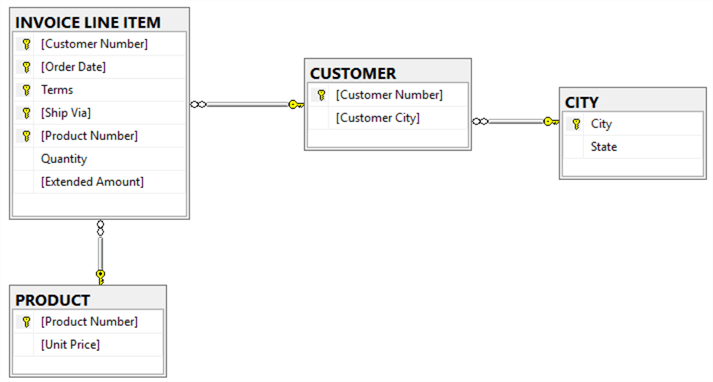
Figure 2 – Entity Relationship Diagram
The objective of normalization is to organize data into normal forms and thereby minimize insert/update/delete anomalies from the data [7]. The normalized relations are beneficial for transaction processing. On the other hand, the normalized data may cause significant inefficiencies in the analytical processing, which infrequently updates data, and always retrieves many rows.
Dimensional Modeling
A dimensional model is a data model structured to deliver maximum query performance and ease of use. A typical dimensional model consists of a fact table surrounding by a set of dimension tables. This data structure is often called a star schema. Dimensional models have proved to be understandable, predictable, extendable, and highly responsive to ad hoc demands because of their predictable symmetric nature [2].
The term fact refers to performance measurements from business processes or events. The invoice, shown in Figure 1, represents a sales activity, the quantity of the product and the extended amount are the measurements of this activity. These numerical facts were “written in stone” once a sales transaction completes. Even if a customer changed an order, a separate business transaction took place, and corresponding measurements were recorded in other fact tables. Thus, data in the fact table is nonvolatile. DBA may update a fact table due to some technical problems. Designers should not consider updating fact tables at design time.
Dimension tables provide context to describe the activity, for example, what was involved in the activity, when, where and why it happened, who perform the activity and how to make it happen. When creating a dimensional model, we should eliminate anything that does not have any business analysis values. For example, the customer phone number is not necessary in the customer dimension.
Kimball introduced a four-step dimensional design process for designing dimensional data models [1][2]. When an entity relationship model is available, we can obtain dimensional models through a four-step transformation process [8]. We use the data captured in the Figure 1 to practice these design processes.
Four-Step Dimensional Design Process
Step 1 – Select the Business Process
A business process is a low-level activity performed by an organization and frequently expressed as action verb [1]. The measurements from each business process are usually represented in a fact table and sometimes several related fact tables [2]. All facts in a fact table should correspond to the same key, in other words, all facts in the fact table should have same granularity and dimensionality. If a fact links to a different key from others, the fact may be from different processes, therefore it should go to other fact table.
The invoice was generated in the business process, selling products. The data collected in the invoice enables business users to analyze sales revenue.
Step 2 – Declare the Grain
The grain exactly specifies the level of detail with the fact table measurements [1]. In the “selling products” activity, the most granular data is every product purchased by a customer.
Step 3 – Identify Dimensions
The grain statement implied the primary dimensionality of the fact tables More dimensions can be added to the fact table if these dimensions naturally take on only one value under each combination of the primary dimensions [6]. Here is a list of dimensions to describe the facts:
(1) Date Dimension
(2) Customer Dimension
(3) Product Dimension
Dimension tables are usually in 2NF and possibly in 3NF, but they cannot be in 1NF. A table in 1NF has partial dependencies, which indicates different entities are mixed into the same dimension table, as demonstrated in Table 2. This introduces the insert anomaly. For example, we cannot add new products to the table if the products have not been sold.
Step 4 – Identify the Facts
In general, fact tables are expressed in 3NF. Typical facts are numeric additive figures. Here is the list of measurements identified in the selected business process.
(1) Quantity
(2) Extended Amount
With results from the four-step process, the dimensional model diagram was shown in the Figure 3.
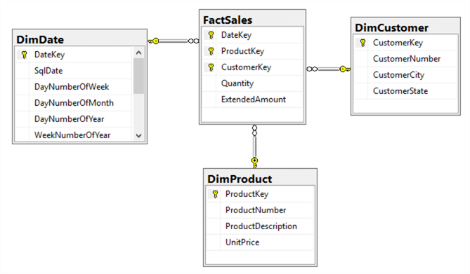
Figure 3 – Dimensional Model Diagram
Four-Step Transformation Process
Several techniques of data warehouse construction from transactional data models have been briefly discussed in [9]. We adopt a four-step process introduced in [8] to convert the 3NF diagram in Figure 2 to a star schema.
Step 1 – Classify entities
In this step, we classify all entities in Figure 2 to three categories:
Transaction Entities: INVOICE LINE ITEM
Component Entities: PRODUCT and CUSTOMER
Classification Entities: CITY
Step 2 – Designing high-level star schema
This step is to designate transaction entities as fact tables and component entities as dimension tables. However, the transaction entity to fact table mapping is not always one-to-one and the correspondence between component entities and dimensions is not always one to one as well. For example, most star schemas include some explicit dimensions, such as date dimension and/or time dimension.
A star schema, shown in Figure 4, can easily be identified from the Figure 2. For complicate diagram, [8] presented a solution with three steps: (1), Identify Star Schemas Required; (2), Define Level of Summarization and (3), Identify Relevant Dimensions.
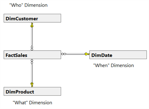
Figure 4 – High-level Star Schema for Selling Product Transaction
Step 3 – Designing detailed fact table
A fact table usually contains a super-key, which consists of degenerate dimensions and all foreign keys linked to dimension tables. The nonprime attributes in the transaction entity can be defined as facts if they have analysis value and they are additive. Figure 5 demonstrates the fact table produced in this step.
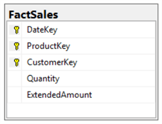
Figure 5 – Fact Table for Selling Product Transaction
Step 4 – Design Detailed Dimension Table
[10] identified and classified four prevalent strategies for denormalization. They are collapsing relations (CR), partitioning a relation (PR), adding redundant attributes (RA), and adding derived attributes (DA). The CR strategy can be used in this step to collapse classification entities into component entities to obtain flat dimension tables with single-part keys that connect directly to the fact table. The single-part key is a surrogate key generated to ensure it remains unique over time. All the dimension tables are presented in Figure 6.
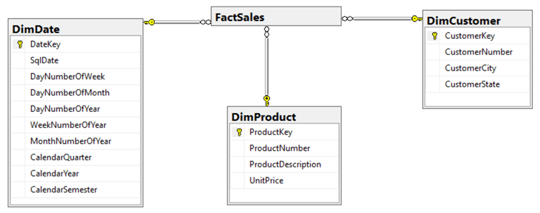
Figure 6 – Dimension Tables for Selling Product Transaction
The star schema obtained from this four-step design process is the same as the one shown in Figure 3. It’s worth noting that dimensional modeling is a mix of science and art. An experienced designer can make a trade-off. The example we used may derive different star schemas. In a summary, ease-of-use and query performance are two primary reasons that dimensional modeling is the widely accepted best practice for data warehousing tools [2]. To achieve the goals, we should resist the temptation to normalize dimension tables.
Reference
[1] Kimball R., and Ross M., The Data Warehouse Toolkit: The Definitive Guide to Dimensional Modeling (3th Edition), Willey, Indiana, 2013.
[2] Ross M., Thornthwaite W., Becker B., Mundy J. and Kimball R., The Data Warehouse Lifecycle Toolkit (2th Edition), Willey, Indiana, 2008.
[3] Wagner J., CSC 455: Database Processing for Large-Scale Analytics, Lecture Note, College of CDM, DePaul University, Chicago, 2017.
[4] Burns L., Building the Agile Database: How to Build a Successful Application Using Agile Without Sacrificing Data Management, Technics Publications, New Jersey, 2011.
[5] Elmasri R., and Navathe S., Fundamentals of Database Systems (4th Edition), Pearson, London, 2003.
[6] Date C. J., An Introduction to Database Systems (8th Edition), Pearson, London, 2003.
[7] Oppel A., Data Modeling A Beginner’s Guide, McGraw-Hill, New York, 2009.
[8] Moody D. L., and Kortink M. A. R., From ER Models to Dimensional Models: Bridging the Gap between OLTP and OLAP Design, Journal of Business Intelligence, vol. 8, 2003.
[9] Dori D., Sturm A. and Feldman R., Transforming an operational system model to a data warehouse model: A survey of techniques, Conference Paper, IEEE Xplore, March 2005.
[10] Shina K. S. and Sandersb L. G., Denormalization strategies for data retrieval from data warehouses, Decision Support Systems 42 (2006) 267– 282
Next Steps
- One purpose of this tip is to compare normalization process (3NF modeling) and dimensional modeling. Dimensional modeling, aiming to analysis processing, is quite different from 3NF modeling. Each of them has own systematic modeling processes and techniques. For more information about normalization, please read Oppel’s book [7]. I strongly recommend Kimball’s books [1][2] for studying dimensional modeling. For more information about converting entity relationship model to dimensional model, please read Moody’s paper [8].
- Shina K. S. and Sandersb L. G. have discussed the denormalization strategies in their paper [10].
- Check out these related tips:

Nai Biao Zhou has twenty years of experience in software development, with strong analytical skills and a broad range of computer expertise.
He has fifteen years of experience in development and maintenance of database applications on SQL Server in OLTP/OLAP/BI environments.
He has a master’s degree in Control Engineering and is pursuing a Master of Science degree in Predictive Analytics.
Knowledge/Skills
Advanced computer programming skills and well versed with C/C#, Java, ASP.NET, JavaScript, and SQL.
In depth knowledge of Solution Architecture, and Software Development Life Cycle (SDLC).
Microsoft Certified Application Developer (MCAD) since 2004.
- MSSQLTips Awards: Author of the Year – 2021 | Rising Star (50+ tips) – 2024 | Author Contender – 2020, 2023