Problem
A SQL Server T-SQL correlated subquery is a special kind of temporary data store in which the result set for an inner query depends on the current row of its outer query. In contrast, an SQL Server T-SQL uncorrelated subquery has the same result set no matter what row is current in its outer query. This section reviews a couple of correlated subquery examples and compares them to alternative formulations based on joins for derived tables. The comparisons rely on an examination of the result sets as well as the execution plans for the alternative formulations. These comparisons shed light on the efficiency of uncorrelated subqueries versus joins between derived tables. The next temporary data store tutorial section will focus more thoroughly on derived tables.
Solution
For the examples below we are using the AdventureWorks2014 database. Download a copy and restore to your instance of SQL Server to test the below scripts.
SQL Server Correlated Subquery as a SELECT List Item
The introduction to subqueries section included coverage of how to use uncorrelated and correlated subqueries as select list items. This section revisits that earlier application of uncorrelated and correlated subqueries from three perspectives.
- First, this section reviews the initial application and presents an alternative approach based on joins instead of subqueries.
- Second, the use of the intersect operator is demonstrated to confirm that the subquery-based and join-based approaches return identical results.
- Third, execution plans for the subquery-based and join-based approaches are contrasted with one another.
Here’s a previously presented code block that demonstrates the use of an uncorrelated subquery and a correlated subquery as items in the select list of a query.
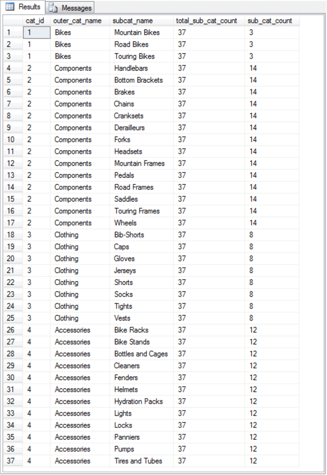
- The first subquery with an alias of total_sub_cat_count is an uncorrelated subquery that returns the count of subcategory values in the join of the ProductCategory and ProductSubcategory tables from the AdventureWorks2014 database. This initial subquery returns the same value for each row of the outer query.
- The other subquery labeled sub_cat_count is a correlated subquery; the return value of this second query depends on the category name value of the outer query. The subquery computes the count of subcategory values within the category for the current row of the outer query. Because there are four product category names in the AdventureWorks2014 database, the correlated subquery returns one of four count values.
-- select list items with uncorrelated and correlated subqueries
SELECT
  outer_cat.ProductCategoryID cat_id,
  outer_cat.Name outer_cat_name,
  subcat.Name subcat_name,
  ( SELECT COUNT(ProductSubcategoryID) subcat_id_count
    FROM [AdventureWorks2014].[Production].[ProductCategory] outer_cat
    INNER JOIN [AdventureWorks2014].[Production].[ProductSubcategory] subcat
       ON outer_cat.ProductCategoryID = subcat.ProductCategoryID
  ) total_sub_cat_count,
  ( SELECT COUNT(ProductSubcategoryID) subcat_id_count
    FROM [AdventureWorks2014].[Production].[ProductCategory] cat
    INNER JOIN [AdventureWorks2014].[Production].[ProductSubcategory] subcat
       ON cat.ProductCategoryID = subcat.ProductCategoryID
    GROUP BY cat.name
    HAVING cat.name = outer_cat.Name
   ) sub_cat_count
FROM [AdventureWorks2014].[Production].[ProductCategory] outer_cat
INNER JOIN [AdventureWorks2014].[Production].[ProductSubcategory] subcat
   ON outer_cat.ProductCategoryID = subcat.ProductCategoryID
It is often possible to reformulate T-SQL queries based on subqueries with joins and WHERE clause criteria. This redesign of a query can eliminate the need for correlated subqueries. Some believe that this reformulation can improve the performance of a query. A good presentation of the issues for and against replacing correlated subqueries with joins appears in this blog (be sure to read comments too). To help evaluate the impact of replacing subqueries with joins, the preceding script sample is re-designed to use joins instead of subqueries. See the next code block for a join-based implementation of the preceding query.
- The first three columns of the query below are from the join of the ProductCategory and ProductSubcategory tables. This code is identical to the preceding query.
- A cross join adds the count of subcategories across categories. When you need to add an identical set values to all rows in another query, then a cross join is a good tool to use. In the example below, the result set from the subcat_id_count subquery is added to the rowset from the join of the ProductCategory and ProductSubcategory tables. The subcat_id_count subquery is used as a derived table.
- A left join adds the result set from the cat_id_count_by_cat_id subquery. The left join through its on clause allows you to specify which result set values from a derived table to apply to which values from the join of the ProductCategory and ProductSubcategory tables.
-- with joins and derived tables
SELECT
  cat.ProductCategoryID cat_id,
  cat.Name cat_name,
  subcat.Name subcat_name,
  subcat_id_count total_sub_cat_count,
  cat_id_count_by_cat_id.cat_id_count_by_cat_id sub_cat_count
FROM [AdventureWorks2014].[Production].[ProductCategory] cat
INNER JOIN [AdventureWorks2014].[Production].[ProductSubcategory] subcat
   ON cat.ProductCategoryID = subcat.ProductCategoryID
CROSS JOIN (
            -- count of subcategories across categories
            SELECT COUNT(ProductSubcategoryID) subcat_id_count
            FROM [AdventureWorks2014].[Production].[ProductSubcategory] subcat
           ) subcat_id_count
LEFT JOIN  (
            -- count of subcategories within categories
            SELECT ProductCategoryID, COUNT(*) cat_id_count_by_cat_id
            FROM [AdventureWorks2014].[Production].[ProductSubcategory] subcat
            GROUP BY ProductCategoryID
           ) cat_id_count_by_cat_id
   ON cat.ProductCategoryID = cat_id_count_by_cat_id.ProductCategoryID
Here are excerpts from the result set with uncorrelated subqueries and correlated subqueries versus the result set for the join-based approach with derived tables.
- The first eleven rows from the subquery approach appear in the top pane.
- Also, the first eleven rows from the join-based approach with derived tables appear in the second pane.
- Each of the two result sets contains thirty-seven rows, but the order of the rows is different, so it is not easy to determine by visual inspection if the two result sets are the same.

The intersect operator is a useful tool for comparing two result sets no matter what the order of rows is in each one. An intersect operator between the result sets for the two approaches returns thirty-seven rows. In other words, the thirty-seven-row result set from each query is identical. The following code block shows how to use the intersect operator to make the comparison.
-- all 37 rows from each query intersect with one another
-- select list items with uncorrelated and correlated subqueries
SELECT
  outer_cat.ProductCategoryID cat_id,
  outer_cat.Name outer_cat_name,
  subcat.Name subcat_name,
  ( SELECT COUNT(ProductSubcategoryID) subcat_id_count
    FROM [AdventureWorks2014].[Production].[ProductCategory] outer_cat
    INNER JOIN [AdventureWorks2014].[Production].[ProductSubcategory] subcat
       ON outer_cat.ProductCategoryID = subcat.ProductCategoryID
  ) total_sub_cat_count,
  ( SELECT COUNT(ProductSubcategoryID) subcat_id_count
    FROM [AdventureWorks2014].[Production].[ProductCategory] cat
    INNER JOIN [AdventureWorks2014].[Production].[ProductSubcategory] subcat
       ON cat.ProductCategoryID = subcat.ProductCategoryID
    GROUP BY cat.name
    HAVING cat.name = outer_cat.Name
   ) sub_cat_count
FROM [AdventureWorks2014].[Production].[ProductCategory] outer_cat
INNER JOIN [AdventureWorks2014].[Production].[ProductSubcategory] subcat
   ON outer_cat.ProductCategoryID = subcat.ProductCategoryID
INTERSECT
-- with joins and derived tables
SELECT
  cat.ProductCategoryID cat_id,
  cat.Name cat_name,
  subcat.Name subcat_name,
  subcat_id_count total_sub_cat_count,
  cat_id_count_by_cat_id.cat_id_count_by_cat_id sub_cat_count
FROM [AdventureWorks2014].[Production].[ProductCategory] cat
INNER JOIN [AdventureWorks2014].[Production].[ProductSubcategory] subcat
   ON cat.ProductCategoryID = subcat.ProductCategoryID
CROSS JOIN ( -- count of subcategories
             SELECT COUNT(ProductSubcategoryID) subcat_id_count
             FROM [AdventureWorks2014].[Production].[ProductSubcategory] subcat
           ) subcat_id_count
LEFT JOIN  ( -- count of subcategories within categories
             SELECT ProductCategoryID, COUNT(*) cat_id_count_by_cat_id
             FROM [AdventureWorks2014].[Production].[ProductSubcategory] subcat
             GROUP BY ProductCategoryID
           ) cat_id_count_by_cat_id
   ON cat.ProductCategoryID = cat_id_count_by_cat_id.ProductCategoryID
The next screen shot displays the thirty-seven rows returned by the intersect operator between the result sets for the two approaches.
- The intersect operator returns a result set which confirms that all thirty-seven rows from each formulation are the same.
- The order of the rows is different, but the intersect operator programmatically matches rows with corresponding column values.
- This correspondence confirms that the subquery-based formulation and the join-based formulation produce identical results.
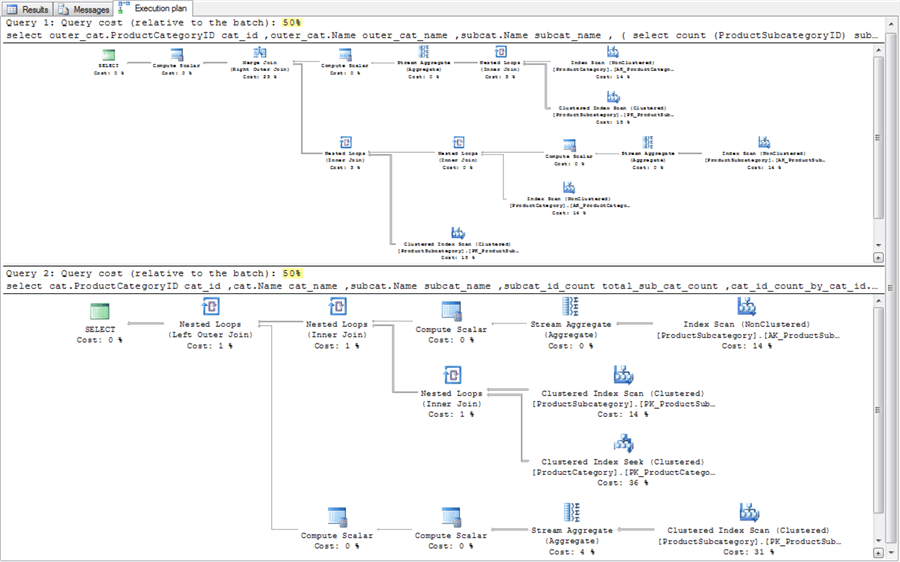
The next screen shot shows the execution plan comparison of the subquery-based and join-based queries.
- The subquery-based execution plan appears above the join-based execution plan.
- The first point to observe is that both query plans have the same execution cost. The two costs are highlighted in the screen shot below.
- In other words, for these two query designs there is no difference in execution cost between the two alternative approaches. Both queries take fifty percent of the relative cost.
- You may be able to discover other subquery-based execution plans with greater costs than join-based execution plans for different source data or slightly different query designs, but for the alternative approaches reviewed in this tutorial section there is no difference.
- In any event, you should consider comparing execution plans whenever there is a concern that one query approach takes longer to run than another approach for the same source data.
- As you can see, the arrangement of operations within each execution plan do vary. Therefore, SQL Server did not perform identical steps to obtain the result set for each query design.
SQL Server Correlated and Uncorrelated Subqueries in WHERE Clauses
While correlated and uncorrelated subqueries can be used for SELECT list items, it is probably more common to encounter them in WHERE clauses for SELECT statements. The code blocks in this tutorial section demonstrate the application of correlated and uncorrelated subqueries in this more usual context. The code samples pull and manipulate data from the AdventureWorks2014 database. This example also requires some pre-processing steps like those needed for any highly normalized production database.
The ultimate goal of the code samples in this section is to list the employees who belong to departments with more than the average number of employees across departments. This is a typical kind of requirement in which you are likely to use correlated or uncorrelated subqueries. The development of the employee list involves
- Compiling a list of employees with such attributes as name, national identifier number, gender, and, of course, department by joining multiple tables and selecting appropriate columns from the source tables
- Computing the count of employees by department as well as the average number of employees across departments
- Linking rows from the list of employees with department name to the count of employees by department as well as the average employee count across departments; this step can be performed with correlated subqueries or joins
- Filtering out, with a where clause, employees who belong to departments with less than or equal to the average number of employees across departments
The code in this tutorial section illustrates subquery-based and join-based approaches to the linking and filtering steps.
The AdventureWorrks2014 tables are representative of those from a production database. The normalized status of many production databases often requires pre-processing before any task can be performed, such as listing the employees who belong to departments with more than the average number of employees across departments.
The following database diagram presents the four AdventureWorks2014 tables used to list the employees who belong to departments with more than the average number of employees across departments.
- Employee first and last names reside in the Person table in the Person schema; the Person table links to the Employee table in the HumanResources schema. The Person table and the Employee table are in a one-to-one relationship.
- Selected employee characteristics, such as gender, job title, and NationalIDNumber, are from the Employee table.
- The Employee and EmploymentDepartmentHistory tables from the HumanResources schema are in a one-to-many relationship in which one employee can belong to different departments in different shifts starting at different dates. As you can see from the diagram, each Employee table row is identified by a BusinessEntityID value, but each EmploymentDepartmentHistory table row is identified by a combination of BusinessEntityID, DepartmentID, ShiftID, and StartDate. Therefore, each BusinessEntityID value can be associated with one or more sets of DepartmentID, ShiftID, and StartDate values.
- For the goal of this example, we only wish to identify an employee with its most recent record in the EmploymentDepartmentHistory table as defined by its StartDate value; this is the most recent department and shift in which an employee worked at the company.
- The department name resides in the Name field of the Department table, which links to the EmploymentDepartmentHistory table by its DepartmentID field.

The following code sample shows a relatively simple query for listing employees from the inner join of the Employee table and the EmployeeDepartmentHistory table. The query returns a single row for each employee, represented by NationalIDNumber, that occurs more than once in the EmployeeDepartmentHistory table. The column values for each row include the NationalIDNumber field value and a count field with an em_count alias.
-- employees with historical membership in more than one department
SELECT
  NationalIDNumber,
  COUNT(edh.BusinessEntityID) em_count
FROM [AdventureWorks2014].[HumanResources].[Employee] em
INNER JOIN [AdventureWorks2014].[HumanResources].EmployeeDepartmentHistory edh
   ON edh.BusinessEntityID = em.BusinessEntityID
GROUP BY NationalIDNumber
HAVING COUNT(edh.BusinessEntityID) > 1
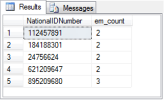
The result set from the preceding query appears below.
- There are five employees who appear more than once in the EmployeeDepartmentHistory table.
- The em_count column values denote the number of times an employee appears in the EmployeeDepartmentHistory table.
- By changing the having clause criterion to “having count(edh.BusinessEntityID) = 1”, you can return a list of employees that occurred just once in the EmployeeDepartmentHistory table. There are 285 employees in this set within the AdventureWorks2014 database.
The next code sample shows an approach to enumerating employees that had more than one row in the EmployeeDepartmentHistory table within the for_mrd derived table. Each employee in the outermost query’s result set has a row with column values for BusinessEntityID and StartDate from the EmployeeDepartmentHistory table, and the most recent date (mrd) for an employee in the EmployeeDepartmentHistory table. The last_value windows function computes the mrd value partitioned by BusinessEntityID. Because a window function cannot be referenced in a WHERE clause, the query with the windows function is nested within an outermost query that receives the value of the windows function along with BusinessEntityID and StartDate value for each row. A WHERE clause in the outermost query selects the row for each employee with a StartDate value equal to the mrd value.
-- most recently worked department for
-- employees who worked in more than one department
-- outer query is required because you cannot use
-- windows function (last_value) in a where clause,
-- but you can assign a windows function an alias (mrd) whose
-- value is referenced in an outer query
SELECT
  BusinessEntityID,
  StartDate,
  mrd
FROM ( SELECT
         edh.BusinessEntityID,
         edh.StartDate,
         edh.DepartmentID,
         LAST_VALUE(startdate) OVER (PARTITION BY edh.BusinessEntityID ORDER BY edh.BusinessEntityID) mrd
       FROM [AdventureWorks2014].[HumanResources].EmployeeDepartmentHistory edh
       WHERE edh.BusinessEntityID IN
               ( -- employees with historical membership in more than one department
                 SELECT  edh.BusinessEntityID
                 FROM [AdventureWorks2014].[HumanResources].[Employee] em
                 INNER JOIN [AdventureWorks2014].[HumanResources].EmployeeDepartmentHistory edh
                    ON edh.BusinessEntityID = em.BusinessEntityID
                 GROUP BY edh.BusinessEntityID
                 HAVING COUNT(edh.BusinessEntityID) >1
                )
     ) for_mrd
WHERE mrd = StartDate
The final pre-processing script builds on the logic from the two preceding queries and the relationships between the AdventureWorks2014 source tables. This query populates the #em_with_dep temp table. The temp table serves as the source table for facilitating the computation of the list the employees who belong to departments with more than the average number of employees across departments. The #em_with_dep temp table has a separate row for each of the 290 employees in the AdventureWorks2014 database. The temp table has more columns than is strictly necessary for deriving a list of employees who come from a department with more than the average number of employees across departments.
The code block below is relatively straightforward in spite of it not being short. The following bullets highlight three major design issues to help readers adapt this kind of code for their purposes.
- Try and catch blocks at the beginning of the script drop any prior version of the #em_with_dep temp table. The remainder of the code in the script populates a fresh version of the temp table.
- The #em_with_dep temp table is populated by a concatenation of rows based on a union operator. The concatenation is for employees that occur just once in the EmployeeDepartmentHistory table followed by the most recent of those that occur more than once in the EmployeeDepartmentHistory table.
- The concatenated result set for the two types of employees is inner joined with the Department table to add department name to the final result set that populates #em_with_dep.
-- populate fresh copy of #em_with_dep
-- containing employees with department membership
-- and other employee attributes (job title and gender)
-- the union operator concatenates two temporary data stores
-- employees who only worked in one department
-- and a second store with employees who worked in more than one deparment
BEGIN TRY
  DROP TABLE #em_with_dep
END TRY
BEGIN CATCH
  PRINT '#em_with_dep is not available to drop'
END CATCH

SELECT
  for_dept_name.*,
  dep.Name dep_name INTO #em_with_dep
FROM ( -- empoyees who worked in one department only
       SELECT
         per.FirstName,
         per.LastName,
         em.BusinessEntityID,
         em.NationalIDNumber,
         em.JobTitle,
         em.Gender,
         edh.DepartmentID
       FROM [AdventureWorks2014].[HumanResources].[Employee] em
       INNER JOIN person.person per
          ON em.BusinessEntityID = per.BusinessEntityID
       INNER JOIN [AdventureWorks2014].[HumanResources].EmployeeDepartmentHistory edh
          ON edh.BusinessEntityID = em.BusinessEntityID
       WHERE em.NationalIDNumber IN
              ( -- employees with historical membership in more than one department
                SELECT
                  NationalIDNumber
                FROM [AdventureWorks2014].[HumanResources].[Employee] em
                INNER JOIN [AdventureWorks2014].[HumanResources].EmployeeDepartmentHistory edh
                   ON edh.BusinessEntityID = em.BusinessEntityID
                GROUP BY NationalIDNumber
                HAVING COUNT(*) = 1
               )

       UNION
       -- most recently worked department (mrd) for
       -- employees who worked in more than one department
       -- and StartDate in department
       SELECT
         per.FirstName,
         per.LastName,
         em.BusinessEntityID,
         em.NationalIDNumber,
         em.JobTitle,
         em.Gender,
         DepartmentID
       FROM ( SELECT
                edh.BusinessEntityID,
                edh.StartDate,
                edh.DepartmentID,
                LAST_VALUE(startdate) OVER (PARTITION BY edh.BusinessEntityID ORDER BY edh.BusinessEntityID) mrd
              FROM [AdventureWorks2014].[HumanResources].EmployeeDepartmentHistory edh
              WHERE edh.BusinessEntityID IN
                  ( -- employees with historical membership in more than one department
                    SELECT edh.BusinessEntityID
                    FROM [AdventureWorks2014].[HumanResources].[Employee] em
                    INNER JOIN [AdventureWorks2014].[HumanResources].EmployeeDepartmentHistory edh
                       ON edh.BusinessEntityID = em.BusinessEntityID
                    GROUP BY edh.BusinessEntityID
                    HAVING COUNT(edh.BusinessEntityID) > 1
                   )
            ) for_mrd
       INNER JOIN [AdventureWorks2014].[Person].[Person] per
          ON per.BusinessEntityID = for_mrd.BusinessEntityID
       INNER JOIN AdventureWorks2014.HumanResources.Employee em
          ON em.BusinessEntityID = per.BusinessEntityID
       WHERE mrd = StartDate
     ) for_dept_name
INNER JOIN AdventureWorks2014.HumanResources.Department dep
   ON dep.DepartmentID = for_dept_name.DepartmentID
-- list employees with department membership
SELECT * FROM #em_with_dep
Here is an excerpt for the list generated by the final select statement in the preceding script. It shows the first 16 rows from the result set from the #em_with_dep temp table. There are 290 rows in total within the table. The remainder of this section shows how to process with either subquery-based techniques or join-based techniques the #em_with_dep temp table to generate a list of the employees belonging to departments with more than the average number of employees across departments.

Here are three basic queries that support computing a list of employees in departments with more than the average number of employees across departments. These queries will subsequently be combined by subquery-based techniques and join-based techniques to achieve the goal of this example. Before illustrating how to combine the queries, let’s examine each query separately.
- The first query computes a count of the number of employees in each department. The syntax uses a group by clause and a count function. The result set contains a separate row for each department with its count of employees.
- The second query is an example of a derived table. The derived table generates the count of employees by department. Its name is em_count_by_dep_name. The count function within the derived table has the alias em_count. The outer query has the #em_with_dep temp table as its source. The select list items in the outer query include a subset of columns from the #em_with_dep temp table along with the em_count column from the derived table.
- The third query computes the average count of employees across departments. It uses a derived table named avg_count_by_dep_name. The avg function in its select list computes the average count across departments. The avg function has the name avg_dep_count.
-- Three basic queries for listing employees that belong
-- to departments with more than the average number of
-- employees across departments
-- employees count by department name
SELECT
  dep_name,
  COUNT(dep_name) em_count
FROM #em_with_dep
GROUP BY dep_name
-- employees with dep_name and em_count_by_department
SELECT
  FirstName,
  LastName,
  Gender,
  JobTitle,
  #em_with_dep.dep_name,
  em_count_by_dep_name.em_count
FROM #em_with_dep
LEFT JOIN
      ( SELECT dep_name, COUNT(dep_name) em_count
        FROM #em_with_dep
        GROUP BY dep_name
      ) em_count_by_dep_name
  ON #em_with_dep.dep_name = em_count_by_dep_name.dep_name
-- avg employees per department
SELECT  AVG(CAST(em_count AS real)) avg_dep_count
FROM
      ( SELECT  COUNT(dep_name) em_count
        FROM #em_with_dep
        GROUP BY dep_name
      ) avg_count_by_dep_name
If you feel the need, you can learn more about the three preceding queries with the following full and partial result set listings.
- There are sixteen departments in the AdventureWorks company. The first query lists the count of employees in each of these departments. As you can see, the Production department has far more employees than any other department.
- The second pane is a partial result set that includes the first seventeen rows from the second query. There are 290 rows in the full result set – one for each employee. This result set shows the outcome of joining the count of employees by department to the list of all employees.
- The third result set has a single row. This is the average count of the number of employees across departments; the average count across departments is 18.125. By comparing the value from this result set to the values from the first result set, you can confirm that just one department – the Production department – has more employees than the average number of employees across departments.

The next script combines the preceding three basic scripts with a correlated subquery and an uncorrelated subquery to compute a list of employees from departments with greater than the average number of employees per department.
- The outermost query is for the #em_with_dep temp table. This query returns employee first and last name along with gender, job title, and department name.
- The temp table is also left joined with a correlated subquery. The correlated subquery name is em_count_by_dep_name. The left join adds the count of the number of employees for a department in which each employee works.
- Next, the left joined result set is filtered through a where clause with the help of an uncorrelated subquery.
- The uncorrelated subquery resides in a derived table named avg_count_by_dep_name.
- The uncorrelated subquery returns the average count of employees across departments.
- The filter retains just those rows from the outermost query’s result set for all employees with a departmental count of employees that is greater than the average count of employees across departments.
- The outermost query’s final select list item references the em_count column from the result set returned by the left join of the correlated subquery to the outermost query.
-- employees from a department with a count
-- greater than the average count per department
-- employees with dep_name and em_count_by_department
-- based on a correlated subquery
SELECT
  FirstName,
  LastName,
  Gender,
  JobTitle,
  #em_with_dep.dep_name,
  em_count_by_dep_name.em_count
FROM #em_with_dep
LEFT JOIN
      ( SELECT dep_name, COUNT(dep_name) em_count
        FROM #em_with_dep
        GROUP BY dep_name
      ) em_count_by_dep_name
  ON #em_with_dep.dep_name = em_count_by_dep_name.dep_name
WHERE em_count_by_dep_name.em_count >
      ( -- avg employees per department
        SELECT AVG(CAST(em_count AS real)) avg_dep_count
        FROM (
               SELECT COUNT(dep_name) em_count
               FROM #em_with_dep
               GROUP BY dep_name
             ) avg_count_by_dep_name
      )
Here’s an excerpt from the result set for the preceding query. It shows the first ten rows from the result set.
- Notice from the row below the Results tab that there are a 179 rows in the full result set. Recall that only one department has more employees than the average number of employees across departments.
- This one department is the Production department, which had an employee count of 179.
- Therefore, all rows in the result set are employees from the Production department. This holds true for the ten rows in the excerpt below as well as the full set of 179 rows in the result set.

Some application developers may find developing solutions with subqueries as a natural process. For example, the preceding query creates a correlated subquery and then left joins it to the outermost query. The left join result set is for all employees. Then, a where clause draws on an uncorrelated subquery with a constraint for only rows for employees with a departmental employee count greater than the average count of employees across departments.
Other application developers may just care to form a joined result set with both the count of the number of employees for the department in which an employee works and the average number of employees across all departments. Then, a filter can be applied to the joined result set that retains only rows where the departmental count for employees is greater than the average count of employees across departments. The following script shows how to develop the application this way.
- As in the preceding solution, a correlated subquery (em_count_by_dep_name) is left outer joined to the outermost query.
- Next, the average count of employees from the avg_count_across_dep subquery is cross joined to the outermost query.
- Finally, the result set based on the left joined and cross joined operations is filtered via a where clause to retain just rows where the departmental count of employees is greater than the average count of employees across departments.
-- employees from a department with a count
-- greater than the average department count
-- based on a left join and a cross join
SELECT
  FirstName,
  LastName,
  Gender,
  JobTitle,
  #em_with_dep.dep_name,
  em_count_by_dep_name.em_count --, avg_count_across_dep.avg_dep_count
FROM #em_with_dep
LEFT JOIN
      (
        SELECT dep_name, COUNT(dep_name) em_count
        FROM #em_with_dep
        GROUP BY dep_name
      ) em_count_by_dep_name
   ON #em_with_dep.dep_name = em_count_by_dep_name.dep_name
CROSS JOIN
      ( -- avg employees per department
        SELECT AVG(CAST(em_count AS real)) avg_dep_count
        FROM (
              SELECT COUNT(dep_name) em_count
              FROM #em_with_dep
              GROUP BY dep_name
             ) avg_count_by_dep_name
      ) avg_count_across_dep
The final query in this tutorial section (see the next script) illustrates the use of the intersect operator to confirm that the join-based solution with a derived table returns the same result set as a subquery-based solution framework. The query returned 179 rows. Recall that 179 is the number of employees in the Production department. Therefore, the join-based and subquery-based approaches return the same set of 179 employees.
-- verify identical outcomes
-- employees from a department with a count
-- greater than the average count per department
-- employees with dep_name and em_count_by_department
-- based on a correlated subquery
SELECT
  FirstName,
  LastName,
  Gender,
  JobTitle,
  #em_with_dep.dep_name,
  em_count_by_dep_name.em_count
FROM #em_with_dep
LEFT JOIN
      ( SELECT dep_name, COUNT(dep_name) em_count
        FROM #em_with_dep
        GROUP BY dep_name
      ) em_count_by_dep_name
   ON #em_with_dep.dep_name = em_count_by_dep_name.dep_name
WHERE em_count_by_dep_name.em_count >
      ( -- avg employees per department
        SELECT AVG(CAST(em_count AS real))
        FROM ( SELECT COUNT(dep_name) em_count
               FROM #em_with_dep
               GROUP BY dep_name
             ) avg_count_by_dep_name
      )
INTERSECT
-- employees from a department with a count
-- greater than the average department count
-- based on a left join and a cross join
SELECT
  FirstName,
  LastName,
  Gender,
  JobTitle,
  #em_with_dep.dep_name,
  em_count_by_dep_name.em_count --, avg_count_across_dep.avg_dep_count
FROM #em_with_dep
LEFT JOIN
      ( SELECT dep_name, COUNT(dep_name) em_count
        FROM #em_with_dep
        GROUP BY dep_name
      ) em_count_by_dep_name
   ON #em_with_dep.dep_name = em_count_by_dep_name.dep_name
CROSS JOIN
      ( -- avg employees per department
        SELECT AVG(CAST(em_count AS real)) avg_dep_count
        FROM (
               SELECT COUNT(dep_name) em_count
               FROM #em_with_dep
               GROUP BY dep_name
             ) avg_count_by_dep_name
      ) avg_count_across_dep
WHERE em_count > avg_dep_count
Is one solution better in the sense that it requires fewer computing resources even though both solutions return the same employees? Also, while the T-SQL code is different between the two approaches, is the SQL Server execution plan the same or different between the two approaches? We can answer both these questions by comparing the execution plans from both solutions.
The following screen shot shows the SQL Server execution plan for the subquery-based approach above and the join-based approach below. There are two main take-aways.
- First, the computing resources were split evenly between the two solutions.
- Second, the reason for this is that SQL Server converted the different code for the two solutions into the exact same execution plan.
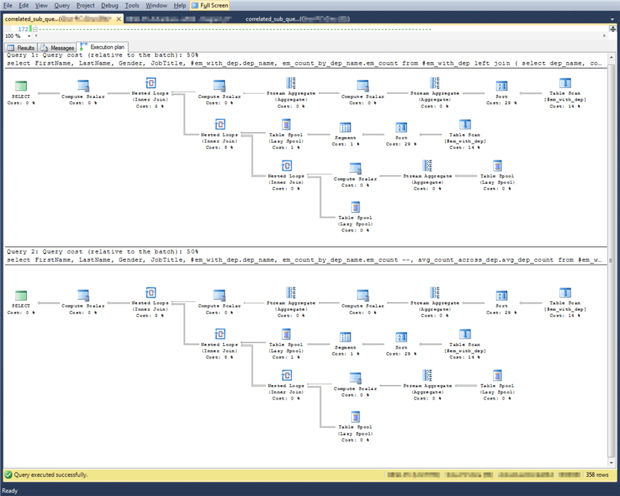
For the SELECT item and WHERE clause examples covered in this tutorial section, there is no difference in resources used between subquery-based solutions and join-based solutions. Furthermore, for the WHERE clause examples, there was not even a difference in the execution plan. Therefore, at least for examples like those covered in this tutorial section, you can freely use either solution strategy. It remains for others to prove with different examples when subquery-based approaches are slower or even materially different in their execution plan than join-based approaches.
Next Steps
Here are some links to resources that you may find useful to help you grow your understanding of content from this section of the tutorial.
- Understanding Correlated and Uncorrelated Sub-queries in SQL
- SQL SERVER – Correlated and Noncorrelated – SubQuery Introduction, Explanation and Example
- A SUB-QUERY DOES NOT HURT PERFORMANCE
- SQL Server Window Function Syntax
- SQL Server Cross Join
- Maximizing your view into SQL Query Plans

Rick Dobson is a SQL Server professional with decades of T-SQL experience that includes authoring books, running a national seminar practice, working for businesses on finance and healthcare development projects, and serving as a regular contributor to MSSQLTips.com. He has been a practicing Python developer for more than the past half decade – with a special emphasis for data visualization and ETL tasks with JSON and CSV files. His most recent professional passions include financial time series data and analyses, AI models, and statistics. If you are interested in growing your skills in any of these areas especially as they relate to financial securities, consider visiting his blog at https://securitytradinganalytics.blogspot.com/2023/12/.
- MSSQLTips Awards: Leadership (200+ tips) – 2025 | Author of the Year Contender – 2017-2024
