Problem
R is a popular data modeling, analysis and plotting framework that can be used to work with data from a variety of sources. In this tip, we will follow on from SQL Server Data Access using R – Part 2 and show some other features of R. We will race a query in a SQL Server 2016 in-memory table against a query on an R data frame; we’ll show how to combine base R functions with package functions; show some new examples of notation; we’ll play around with in-memory settings, and we’ll show how to map data points to world maps in R and in SSRS.
Solution
Configuring the Environment
If you haven’t done so already, you’ll need to follow the steps in SQL Server Data Access Using R – Part 1 to install and configure your R/RStudio environment.
For this tip, we’ll be using SQL Server 2016 Developer Edition. This is available free from Microsoft, following registration with the Visual Studio Dev Essentials program, at the following URL: https://www.microsoft.com/en-us/sql-server/application-development
You’ll also need to be working on a machine with a sufficient amount of memory available to SQL Server – I would recommend at least 2GB.
SQL Server vs. R
The first thing we’ll do is look at the comparative performance of a SQL Server 2016 in-memory table versus querying an R data frame. Both structures are held in-memory, and SQL Server has the benefit of being able to use indexes to help query performance. For in-memory tables, only hash indexes or non-clustered indexes can be used. The entries in an index on a memory-optimised table are also held in memory (the index isn’t disk-based), and rather than looking up the key value in a normal disk-based index, the in-memory index entries are direct memory addresses for the relevant data. This can make a SQL Server in-memory index an extremely powerful tool. We’ll test query execution times against both in-memory tables without a corresponding index, and in-memory tables with an index.
Unlike SQL Server, R does not support indexing data frames. Indeed, the word ‘index’ is used very differently – it means to address data. So, one may use index [2] to identify the second column in a data frame, or we can also index by row. It roughly corresponds to the way in which we SELECT certain columns or use WHERE filters to include rows in SQL. However, R benefits from an extremely simple underlying implementation of data frames where there isn’t the overhead of the parser, algebrizer or optimizer found in the SQL Server database engine, which makes it a good competitor to SQL Server in this context, as we’ll see.
In the last tip, we promised not to use AdventureWorks again – so, for this tip, we’ll use a publicly-available and much more interesting dataset – details of crimes committed in the city of Chicago from 2001 to the present day. This is available in CSV format free of charge and without registration here: https://data.cityofchicago.org/api/views/ijzp-q8t2/rows.csv?accessType=DOWNLOAD. This dataset is around 1.4GB in size and is structured as follows. There are improvements available to the data types chosen but these will do for the purposes of the tip:

Once you have downloaded this data, we’ll import it into SQL Server into a memory-optimised table. Create the following format file in your C:\TEMP directory and call it ‘chicagoFF.fmt’:
<?xml version="1.0"?>
<BCPFORMAT
 xmlns_xsi="http://www.w3.org/2001/XMLSchema-instance">
  <RECORD>
     <FIELD ID="1" xsi_type="CharTerm" TERMINATOR="," MAX_LENGTH="12"/>
     <FIELD ID="2" xsi_type="CharTerm" TERMINATOR="," MAX_LENGTH="20" COLLATION="SQL_Latin1_General_CP1_CI_AS"/>
     <FIELD ID="3" xsi_type="CharTerm" TERMINATOR="," MAX_LENGTH="22"/>
     <FIELD ID="4" xsi_type="CharTerm" TERMINATOR="," MAX_LENGTH="250" COLLATION="SQL_Latin1_General_CP1_CI_AS"/>
     <FIELD ID="5" xsi_type="CharTerm" TERMINATOR="," MAX_LENGTH="10" COLLATION="SQL_Latin1_General_CP1_CI_AS"/>
     <FIELD ID="6" xsi_type="CharTerm" TERMINATOR="," MAX_LENGTH="250" COLLATION="SQL_Latin1_General_CP1_CI_AS"/>
     <FIELD ID="7" xsi_type="CharTerm" TERMINATOR="," MAX_LENGTH="250" COLLATION="SQL_Latin1_General_CP1_CI_AS"/>
     <FIELD ID="8" xsi_type="CharTerm" TERMINATOR="," MAX_LENGTH="250" COLLATION="SQL_Latin1_General_CP1_CI_AS"/>
     <FIELD ID="9" xsi_type="CharTerm" TERMINATOR="," MAX_LENGTH="5" COLLATION="SQL_Latin1_General_CP1_CI_AS"/>
     <FIELD ID="10" xsi_type="CharTerm" TERMINATOR="," MAX_LENGTH="5" COLLATION="SQL_Latin1_General_CP1_CI_AS"/>
     <FIELD ID="11" xsi_type="CharTerm" TERMINATOR="," MAX_LENGTH="50" COLLATION="SQL_Latin1_General_CP1_CI_AS"/>
     <FIELD ID="12" xsi_type="CharTerm" TERMINATOR="," MAX_LENGTH="100" COLLATION="SQL_Latin1_General_CP1_CI_AS"/>
     <FIELD ID="13" xsi_type="CharTerm" TERMINATOR="," MAX_LENGTH="100" COLLATION="SQL_Latin1_General_CP1_CI_AS"/>
     <FIELD ID="14" xsi_type="CharTerm" TERMINATOR="," MAX_LENGTH="100" COLLATION="SQL_Latin1_General_CP1_CI_AS"/>
     <FIELD ID="15" xsi_type="CharTerm" TERMINATOR="," MAX_LENGTH="100" COLLATION="SQL_Latin1_General_CP1_CI_AS"/>
     <FIELD ID="16" xsi_type="CharTerm" TERMINATOR="," MAX_LENGTH="12"/>
     <FIELD ID="17" xsi_type="CharTerm" TERMINATOR="," MAX_LENGTH="12"/>
     <FIELD ID="18" xsi_type="CharTerm" TERMINATOR="," MAX_LENGTH="5"/>
     <FIELD ID="19" xsi_type="CharTerm" TERMINATOR="," MAX_LENGTH="22"/>
     <FIELD ID="20" xsi_type="CharTerm" TERMINATOR="," MAX_LENGTH="14"/>
     <FIELD ID="21" xsi_type="CharTerm" TERMINATOR="," MAX_LENGTH="14"/>
     <FIELD ID="22" xsi_type="CharTerm" TERMINATOR="\n" MAX_LENGTH="250" COLLATION="SQL_Latin1_General_CP1_CI_AS"/>
  </RECORD>
  <ROW>
     <COLUMN SOURCE="1" NAME="ID" xsi_type="SQLINT"/>
     <COLUMN SOURCE="2" NAME="Case_Number" xsi_type="SQLVARYCHAR"/>
     <COLUMN SOURCE="3" NAME="Date" xsi_type="SQLDATETIME"/>
     <COLUMN SOURCE="4" NAME="Block" xsi_type="SQLVARYCHAR"/>
     <COLUMN SOURCE="5" NAME="IUCR" xsi_type="SQLVARYCHAR"/>
     <COLUMN SOURCE="6" NAME="Primary_Type" xsi_type="SQLVARYCHAR"/>
     <COLUMN SOURCE="7" NAME="Description" xsi_type="SQLVARYCHAR"/>
     <COLUMN SOURCE="8" NAME="Location_Description" xsi_type="SQLVARYCHAR"/>
     <COLUMN SOURCE="9" NAME="Arrest" xsi_type="SQLVARYCHAR"/>
     <COLUMN SOURCE="10" NAME="Domestic" xsi_type="SQLVARYCHAR"/>
     <COLUMN SOURCE="11" NAME="Beat" xsi_type="SQLVARYCHAR"/>
     <COLUMN SOURCE="12" NAME="District" xsi_type="SQLVARYCHAR"/>
     <COLUMN SOURCE="13" NAME="Ward" xsi_type="SQLVARYCHAR"/>
     <COLUMN SOURCE="14" NAME="Community_Area" xsi_type="SQLVARYCHAR"/>
     <COLUMN SOURCE="15" NAME="FBICode" xsi_type="SQLVARYCHAR"/>
     <COLUMN SOURCE="16" NAME="XCoordinate" xsi_type="SQLINT"/>
     <COLUMN SOURCE="17" NAME="YCoordinate" xsi_type="SQLINT"/>
     <COLUMN SOURCE="18" NAME="Year" xsi_type="SQLSMALLINT"/>
     <COLUMN SOURCE="19" NAME="Updated_On" xsi_type="SQLDATETIME"/>
     <COLUMN SOURCE="20" NAME="Latitude" xsi_type="SQLDECIMAL" PRECISION="12" SCALE="9"/>
     <COLUMN SOURCE="21" NAME="Longitude" xsi_type="SQLDECIMAL" PRECISION="12" SCALE="9"/>
         <COLUMN SOURCE="22" NAME="Location" xsi_type="SQLVARYCHAR"/>
  </ROW>
</BCPFORMAT>
Note: To use memory optimized structures in SQL Server, you must first have a memory optimized filegroup with a file associated to it. Here is some sample code against a ‘DBA’ database to create such a structure – amend the parameters to suit your environment.
ALTER DATABASE DBA ADD FILEGROUP inmem CONTAINS MEMORY_OPTIMIZED_DATA
ALTER DATABASE DBA ADD FILE (name = 'inmem', filename = 'c:\temp\inmem.ndf') TO FILEGROUP inmem
Now create the following (on-disk) table in SQL Server:
CREATE TABLE chicago (
   ID INT PRIMARY KEY,
   Case_Number VARCHAR(20), [Date] DATETIME, [Block] VARCHAR(250),
   IUCR VARCHAR(10), Primary_Type VARCHAR(250), [Description] VARCHAR(250),
   Location_Description VARCHAR(250), Arrest VARCHAR(5), Domestic VARCHAR(5), Beat VARCHAR(50),
   District VARCHAR(100), Ward VARCHAR(100), Community_Area VARCHAR(100),
   FBICode VARCHAR(100), XCoordinate INT, YCoordinate INT, [Year] SMALLINT,
   Updated_On DATETIME, Latitude NUMERIC(12,9), Longitude NUMERIC(12,9), [Location] VARCHAR(250) )
GO
Now make sure you’ve saved your format file (above), and import the data from the CSV file like so. Feel free to amend the parameters to suit – i.e. the location of the downloaded dataset.
Note, MAXERRORS is set high, as the dataset is polluted with field data containing commas – this, as any seasoned BI dev will tell you, is anathema in CSV files! We’ll simply discard the rows that error out as we don’t really care about these for the purposes of this tip. The row count after discarding bad rows is approximately 6.1m.
BULK INSERT chicago
FROM N'C:\temp\Crimes_-_2001_to_present.csv'
WITH (FORMATFILE = N'C:\TEMP\ChicagoFF.fmt',
      FIRSTROW=2,
      MAXERRORS=10000000 )
GO
Now we’ll create a memory-optimized version of this table called ‘chicagoMO’ and skim the first 250k rows by latest date off the main ‘chicago’ dataset and into memory. Let’s create a non-clustered index on the table to help, then create the memory-optimized table:
CREATE NONCLUSTERED INDEX ncix_chicago_date ON chicago([Date], ID)
CREATE TABLE chicagoMO (
   ID INT PRIMARY KEY NONCLUSTERED,
   Case_Number VARCHAR(20), [Date] DATETIME, [Block] VARCHAR(250),
   IUCR VARCHAR(10), Primary_Type VARCHAR(250), [Description] VARCHAR(250),
   Location_Description VARCHAR(250), Arrest VARCHAR(5), Domestic VARCHAR(5), Beat VARCHAR(50),
   District VARCHAR(100), Ward VARCHAR(100), Community_Area VARCHAR(100),
   FBICode VARCHAR(100), XCoordinate INT, YCoordinate INT, [Year] SMALLINT,
   Updated_On DATETIME, Latitude NUMERIC(12,9), Longitude NUMERIC(12,9), [Location] VARCHAR(250) )
   WITH (MEMORY_OPTIMIZED=ON)
GO
INSERT INTO chicagoMO
   SELECT   TOP 250000 *
   FROMchicago
   ORDERBY [Date] DESC

SELECT TOP 100 * FROM chicagoMO

Now, let’s import the same 250k subset of data into a data frame in R from the chicagoMO table in SQL Server. Execute the following code in RStudio to achieve this. Note you will need to install the relevant packages if not already installed – code supplied to do this – omit this code if not necessary, and change the connection string to suit your environment.
install.packages("RODBC")
install.packages("dplyr")
install.packages("sqldf")
library("RODBC")
library("dplyr")
library("sqldf")
conn <- odbcDriverConnect('driver={SQL Server};server=localhost\\SANDBOX;database=DBA;Trusted_Connection=true;')
chicagoData <- sqlQuery(conn, "SELECT * FROM DBA.dbo.chicagoMO")
chicagoData <- as.data.frame(chicagoData)
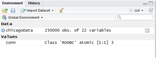
Now before we play with the data, let’s learn something about the internal representation of this data in R. An R data frame isn’t a table in the relational sense. It is a special case of a list, on which a large variety of methods can be executed. We can use the pryr package to poke around at our new data frame, and try to understand a little about how it is stored and how much memory it occupies. Let’s start with object_size():
install.packages("pryr")
library("pryr")
pryr::object.size(chicagoData)
Object.size() is reporting 54MB used for this data. If we divide 54MB by 250,000 rows, we get 221 bytes per row on average, or 10 bytes per column on average, which seems reasonable. We can also use this information plus a bit of mathematics to estimate how many bad rows we dropped earlier: if 54MB = 250k rows, then roughly 216MB is occupied for every 1m rows. We know the original dataset came in at around 1,400MB so, divide 1400MB / 216MB to yield 6.48m rows. We currently have 6.1m rows in the original data set, so (6.4 – 6.1) * 100 = approximately 4.6% of rows contained commas, and were dropped.
We can see how much memory R is using overall, for all objects, by using mem_used(), which can be useful if we’re working with multiple result sets in our environment:

We’re using a notation now that we didn’t use before: <package>::. When we estimated object.size(), we called it from the pryr package – the object.size() method actually already exists in base R. We can refer to a specific package by using this notation to tell R we want to call the version of the method that belongs to that package, and not any other package using this notation.
So, we have this data – let’s compose some interesting questions.
- Question A: What was the most common type of crime in Chicago in January 2017?
- Question B: What is most likely, overall – that I will be robbed, or my home will be burgled?
- Question C: Which are the most crime-ridden areas of Chicago?
Answering Question A
First -we can get this information from SQL with ease by simply grouping the data by Primary_Type and counting the types. We can also group this data in R using the techniques shown in Part 1 and Part 2 of this tip series to achieve the same outcome. But, which is faster?
SET DATEFORMAT YMD
SELECT   Primary_Type, COUNT(*) [Occurrences]
FROM chicagoMO
WHERE [Date] BETWEEN '2017-01-01' AND '2017-01-31'
GROUP BY Primary_Type
ORDER BY COUNT(*) DESC
OPTION (RECOMPILE)

Okay, that took a surprisingly long time – 7.3 seconds. Our in-memory SQL table is not indexed, which could account for the delay as a table scan of the 250,000-strong data set would be required to search the [Date] column.
Let’s try it in R, using a mix of base R and dplyr, which we learned about in Part 2 of this tip series. We can achieve exactly the same result like this:
startTime <- proc.time()
qA <- chicagoData[chicagoData$Date >= "2017-01-01" & chicagoData$Date <= "2017-01-31",];
qA <- table(qA$Primary_Type) %>% as.data.frame();
qA <- arrange(qA, desc(qA$Freq));
endTime <- proc.time()
duration <- endTime - startTime
Some more notation here. We have filtered the chicagoData data set using two primitive expressions – we can do this using the square bracket [ ] notation without using anything more complicated like dplyr. Square brackets are used to extract data from other data – here, we have asked for data where the Date column falls between two dates, and crucially (see the comma at the end?) all other data too.
We’re also using a new base R function called table – this is a very simple way of grouping by a column with a frequency count. It’s actually a little more powerful than this – you can read more about it by executing this ?table.
After filtering and grouping the data, we sort it in descending order. Finally, the whole process is timed.
Let’s examine the output objects:
| SQL Server | R |
|---|---|
 |  |
We’re not actually achieving the same results here – there’s a slight variation, which could be due to the differences between the date evaluation on a date type between SQL Server and R, since we used BETWEEN in one context and >= / <= in the other. However, they are roughly the same which is good enough for our example, so let’s proceed anyway, and examine the duration variable in the Environment Window in R to see how long the operation took:

Wow – this is measured in seconds – the whole R operation took just 60ms to return, compared with over 7 seconds for a SQL Server memory optimized table.
Here’s what is extraordinary – when we repeat the SQL code to reproduce the results, this consistently takes over 7 seconds to return – and 73% of the time is taken on the table scan (in memory). Whereas R is consistently returning the same result in under a tenth of a second! We’re also doing exactly the same thing in the same order – filtering the table by date, aggregating it, sorting it and returning it. Here’s the SQL execution plan:

And we won’t show it here, but the estimated I/O cost is nil, and there’s little I/O activity going on at the same time – this is definitely happening in-memory.
In this test, at least, R has comprehensively beaten SQL Server.
Answering Question B
About the higher likelihood in Chicago – robbery, or burglary – requires a slightly different query. Here are the SQL Server and R versions side-by-side:
SQL Server:
SET DATEFORMAT YMD
SELECT TOP 1 'You are more likely to be a victim of ' + UPPER(Primary_Type) [Occurrences]
FROM chicagoMO
WHERE Primary_Type IN ('ROBBERY','BURGLARY')
GROUP BY Primary_Type
ORDER BY COUNT(*) DESC
OPTION (RECOMPILE)
R:
startTime <- proc.time()
qB <- chicagoData[chicagoData$Primary_Type %in% c("ROBBERY","BURGLARY"),];
qB <- table(qB$Primary_Type) %>% as.data.frame();
qB <- arrange(qB, desc(qB$Freq));
result <- subset.data.frame(head(qB, n=1))
print(paste("You are more likely to be a victim of",as.character(result$Var1)))
endTime <- proc.time()
duration <- endTime - startTime
duration
Both queries return the same result:

But SQL Server returned in 8.6 seconds – and R returned in just 230ms. Once again, R has outperformed SQL Server. Checking the execution plan, we do see a spillage to tempdb this time – the SQL instance ran out of memory to deal with the computation – we’ll find out why in a moment. However, 8.6 seconds is still a very long time to wait.
Let’s repeat the experiment but in SQL Server, we’ll try to add a new hash index on [Primary_Type] to enable the query to function faster:
ALTER TABLE chicagoMO
ADD INDEX ncix_chicagoMO_Primary_Type HASH (Primary_Type) WITH (BUCKET_COUNT = 8);
But … wait a minute!
My instance has run out of memory. Given that right now, I have nothing else going on in SQL Server and no other memory-optimised tables, let’s take a look and see how much space the memory optimized table is taking up:

The table itself is taking up the expected amount of room – nearly identical to R. When I examine the memory usage on the server, we find 2.1GB allocated to SQL Server – not excessive. So we’ve blown the default pool – let’s check, do we need to use a different pool?
“To protect SQL Server from having its resources consumed by one or more memory-optimized tables, and to prevent other memory users from consuming memory needed by memory-optimized tables, you should create a separate resource pool to manage memory consumption for the database with memory-optimized tables.” Read more here : https://docs.microsoft.com/en-us/sql/relational-databases/in-memory-oltp/bind-a-database-with-memory-optimized-tables-to-a-resource-pool
Ah.
Okay, let’s follow the instructions – the database already exists, so let’s create a new resource pool, bind the database to it and bounce the database to activate it:
CREATE RESOURCE POOL Pool_DBA
WITH
   ( MIN_MEMORY_PERCENT = 50,
     MAX_MEMORY_PERCENT = 50 );
GO
ALTER RESOURCE GOVERNOR RECONFIGURE;
GO
EXEC sp_xtp_bind_db_resource_pool 'DBA', 'Pool_DBA'
GO
ALTER DATABASE DBA SET OFFLINE WITH ROLLBACK IMMEDIATE;
ALTER DATABASE DBA SET ONLINE;
Now let’s retry our index:
ALTER TABLE chicagoMO
ADD INDEX ncix_chicagoMO_Primary_Type HASH (Primary_Type) WITH (BUCKET_COUNT = 8);
And re-execute our Question B test query:
SET DATEFORMAT YMD
SELECT TOP 1 'You are more likely to be a victim of ' + UPPER(Primary_Type) [Occurrences]
FROM chicagoMO
WHERE Primary_Type IN ('ROBBERY', 'BURGLARY')
GROUP BY Primary_Type
ORDER BY COUNT(*) DESC
OPTION (RECOMPILE)
Which executes in:

Wow – well, it looks like removing the table scan sorted out the delay! It appears R’s filter and sort methods are top-of-the range – but SQL Server wins this round, with 171ms (including a full recompilation).
Answering Question C
This is rather difficult – which are the most crime-ridden areas of Chicago?
This is a very subjective question. How do we measure ‘most’? Is this simply a descending-order query? Luckily, the data set owners have provided latitude and longitude measurements for every crime listed. Instead of racing, let’s show how we can plot this data as a set of points on to a map in SQL Server Reporting Services. We can also use the rworldmap package to do the same in R.
First, let’s create a new on-disk table to contain a list of the lat/long points in the GEOGRAPHY data type, along with the frequency that they occur.
CREATE TABLE chicagoLocations ( lat DECIMAL(12,9), long DECIMAL(12,9), loc GEOGRAPHY, freq INT )
GO
INSERT INTO chicagoLocations
   SELECT   latitude, longitude, NULL, COUNT(*)
   FROM chicago
   WHERE latitude IS NOT NULL AND longitude IS NOT NULL
   GROUP BY latitude, longitude
select COUNT(*) from chicagoLocations
UPDATE chicagoLocations
SET loc = geography::Parse('POINT(' + CAST([long] AS VARCHAR(20)) + ' ' +
    CAST([lat] AS VARCHAR(20)) + ')')
We now have a chicagoLocations table containing spatial data points and the number of crimes committed at each location. For more information on the GEOGRAPHY data type, see Next Steps.
In SQL Server Data Tools (SSDT), let’s create a new Report Services Project using the Wizard like so, and call it ChicagoMap:

Space is limited here to step through map creation in SSRS step by step, so we can use the excellent article by Brady Upton on MSSQLTips (https://www.mssqltips.com/sqlservertip/2552/creating-an-ssrs-map-report-with-data-pinpoints/ ) to help us achieve this. Follow Brady Upton’s instructions to create a basic map from the States by County drilldown for Illinois, and tick the box for a Bing Maps overlay. Modify Brad’s instructions and use a Bubble Map, and use the chicagoLocations dataset (ignoring ID), and you should (after a couple of attempts) get something that looks similar to the following:

We can see that the west side has a much greater proportion of crimes than the east coast!
So we’ve established SQL Server has mapping capabilities – what about R?
In R, we can use a few packages – ggmap, which wraps map and ggplot2 to render maps, and mapproj. Together, these will allow us to query Google Maps and render any area of the world as a ggplot object.
First, we’ll need to get our ChicagoLocations data into R. Use the following code. Note that we are using a different driver – the SQL Server Native Client. Why? Because the standard ODBC SQL Server driver won’t deal with VARBINARY or spatial data types like GEOGRAPHY (and my thanks to Steph Locke for helping me diagnose this issue last week!)
conn <- odbcDriverConnect('driver={SQL Server Native Client 11.0};server=localhost\\SANDBOX;database=DBA;Trusted_Connection=yes;')
chicagoLocations <- sqlQuery(conn, "SELECT * FROM DBA.dbo.chicagoLocations")
chicagoLocations <- as.data.frame(chicagoLocations)
All we’re doing here is creating a data frame containing our location data from chicagoLocations.
Next, create a new object called chicagoMap. This, to begin with, will contain a map of Chicago zoomed in to an appropriate level from Google Maps. Zoom levels are 0 (world) to 21 (building).
install.packages("ggmap")
install.packages("mapproj")
install.packages("maps")
library(ggmap)
library(mapproj)
library(maps)
chicagoMap <- get_map(location = 'Chicago', zoom = 10)
chicagoMap <- ggmap(chicagoMap)
Typing ggmap(chicagoMap) renders the map into the plot window to the right. If it doesn’t, or you receive a blank screen, type install.packages(“maps”) and let the maps package install, then restart R. Don’t forget to reload your libraries. You should have something that looks like this:

Now, we need to overlay our latitude and longitude points onto the map. We can do this like so. Check back with Part 1 for an introduction to ggplot2 – all we’re doing is grabbing our latitude and longitude points, and creating a scale against frequency in a points- type of plot.
ggmap(chicagoMap) + geom_point(data=chicagoLocations, aes(x=long, y=lat), size=1)

In this map, size =1 and transparency is 0% so there’s no indication of frequency (i.e. by using a bubble map). This presents a bit of a problem – the map above is fairly useless, as it only indicates there was a crime in any given area, not how frequent they were. To help solve this we can try a bit of maths.
Now, we know the minimum frequency of crime in a given location is 1, and with a simple SQL SELECT query against chicagoLocations (in SQL Server) we can check the maximum:
SELECT max(freq) FROM chicagoLocations

Now size = 1 in geom_point as a constant will render a small point. Let’s take this as a minimum – with the maximum as 12,036, this size point is no good, it’s too big and will obliterate the map. We need to map frequency to point size, and make it realistic. A linear function will work here, but we’ll spell it out as a CASE statement to make it clear. Let’s pick an arbitrary range for our point size – say, 1-10. So, dividing the maximum by the number of boundaries (10) yields a ‘step’ of 1,200. At each step, we’ll increase bubble size by 1.
Let’s add a column to our chicagoLocations table using SQL, a series of CASE statements that will map bubble size like so:
ALTER TABLE chicagoLocations ADD bubbleSize TINYINT
UPDATE chicagoLocations SET bubbleSize =
   CASE  WHEN freq >= 1 AND freq <= 1200 THEN 1
         WHEN freq > 1200 AND freq <= 2400 THEN 2
         WHEN freq > 2400 AND freq <= 3600 THEN 3
         WHEN freq > 3600 AND freq <= 4800 THEN 4
         WHEN freq > 4800 AND freq <= 6000 THEN 5
         WHEN freq > 6000 AND freq <= 7200 THEN 6
         WHEN freq > 7200 AND freq <= 8400 THEN 7
         WHEN freq > 8400 AND freq <= 9600 THEN 8
         WHEN freq > 9600 AND freq <= 10800 THEN 9
         WHEN freq > 10800 AND freq <= 12036 THEN 10
   END
And we will rerun our R code to re-import the data with our extra column:
chicagoLocations <- sqlQuery(conn, "SELECT * FROM DBA.dbo.chicagoLocations")
chicagoLocations <- as.data.frame(chicagoLocations)
chicagoMap <- get_map(location = 'Chicago', zoom = 10)
ggmap(chicagoMap) + geom_point(data=chicagoLocations,
                    aes(x=long, y=lat, size=bubbleSize), alpha=0.1, colour="Red")
chicagoMap
Note we are setting transparency using alpha – a 0-1 measure indicating transparency, where 1 is opaque.

This map is not much better! However, we’re mapping by frequency, not by a constant and if you look at the top left portion of the plot, you can see this more clearly. We have made progress. However in SSRS, we had graded colour to help illustrate the data. Let’s add one more column to our chicagoLocations table – this one with hex values indicating ten steps of colour:
ALTER TABLE chicagoLocations ADD colour VARCHAR(7)
UPDATE chicagoLocations SET colour =
   CASE WHEN bubbleSize = 1 THEN '#00ff00'
   WHEN bubbleSize = 2 THEN '#66ff66'
   WHEN bubbleSize = 3 THEN '#99ff66'
   WHEN bubbleSize = 4 THEN '#ccff66'
   WHEN bubbleSize = 5 THEN '#ffff66'
   WHEN bubbleSize = 6 THEN '#ffcc00'
   WHEN bubbleSize = 7 THEN '#cc6600'
   WHEN bubbleSize = 8 THEN '#993300'
   WHEN bubbleSize = 9 THEN '#990000'
   WHEN bubbleSize = 10 THEN '#800000'
   END
And when we modify the ggmap call in the R code like this:
ggmap(chicagoMap) + geom_point(data=chicagoLocations,
                    aes(x=long, y=lat, size=bubbleSize, colour=chicagoLocations$colour),
                    alpha=0.1)
We get a slightly better map indicating crime frequency by colour and size, although the frequency is high:

So, what’s the problem? Let’s roughly model the distribution in SQL:
SELECT bubbleSize * 1200 [approx_range], COUNT(*) [occurrences]
FROM chicagoLocations
GROUP BY bubblesize * 1200
ORDER BY COUNT(*) DESC

We’ve found the problem. The lat and long measurements are so precise that nearly all the frequencies of crime are lower than 1,200 per data point – in other words, we have a grossly skewed distribution.
We would need to experiment with reformatting our colour and bubble sizes to fit the data. One problem is that we are modelling 800,000 data points here using relatively large circles – the overlays make seeing the crime extents difficult. We have a number of options to solve this, which we won’t pursue for now, but should give you some ideas – we could randomly sample the data, reducing the data points down to a manageable number; we could alter our colour mappings to better reflect the spread of the distribution in the frequency data; we could cluster the data around e.g. 30-50 centres using techniques like k-means; we could use different aesthetics to render the data; we could split the map up into districts by incorporating shapefiles instead of Google Maps; and so on.
The verdict in a nutshell – SSRS is much more straightforward and user-friendly when creating maps, but R is much more configurable. With large or complex data sets, SSRS wins this round for sheer visual appeal and user-friendliness.
That’s the end of this tip. We’ve shown by example how to import data to R from SQL Server; how to set up in-memory tables; had a ‘fun run’ where we paced R vs. SQL Server on SELECT execution performance; we have learned about table in R, about using square bracket notation, and how to plot maps both in SSRS and in R.
In the next tip, we’ll use the same Chicago dataset but this time show how to convert each record (row) into a MongoDB document. We’ll show how to configure a new MongoDB collection in Azure (CosmosDB) and connect using R. We’ll convert on-the-fly from tabular to JSON format, then show how to extract the JSON from MongoDB and store (and query!) it as JSON in SQL Server. We’ll play with MongoDB Compass, the client tool for MongoDB, and maybe have a SQL Server vs. MongoDB JSON query retrieval race. Check back soon!
Next Steps
- Further reading:
- Brad Upton – Creating an SSRS Map Report with Data Pinpoints – https://www.mssqltips.com/sqlservertip/2552/creating-an-ssrs-map-report-with-data-pinpoints/
- Siddharth Mehta – Create Custom Maps for SQL Server Reporting Services SSRS Mobile Reports – https://www.mssqltips.com/sqlservertip/4704/create-custom-maps-for-sql-server-reporting-services-ssrs-mobile-reports/
- Microsoft – Indexes for Memory-Optimized Tables – https://docs.microsoft.com/en-us/sql/relational-databases/in-memory-oltp/indexes-for-memory-optimized-tables
- Plot.ly – Plotting bubble maps in R – https://plot.ly/r/bubble-maps/

Dr. Derek Colley is the lead technical consultant for Optimal Computing, a boutique data consultancy based in the UK NW helping clients troubleshoot, configure, plan and deploy their data platforms. He specializes in data integration and database performance optimization, and is a PhD candidate with Staffordshire University, looking into methods of integrating AL query selection algorithms with the cost-based query optimizer. In his spare time, he enjoys building robots, going outdoors, and spending time with his four children.
- MSSQLTips Awards: Trendsetter (25+ tips)