Problem
I heard that weighted moving averages are better than simple moving averages for tracking recent values in time series data. Yet, I know from a prior tip that simple moving averages are easy to compute with the Windows aggregate avg function. Please present computational techniques for a couple of different types of weighted moving averages. Also, present some simple examples comparing the relationship of simple moving averages and weighted moving averages for the same underlying time series values.
Solution
Moving averages are useful for smoothing out the random variations from period to period in a set of time series values. While it is relatively easy and efficient to compute simple moving averages with the Windows aggregate avg function, there is no Windows aggregate function for computing weighted moving averages. This tip presents T-SQL code for computing two different types of weighted moving averages for time series data.
- One common weighted moving average is called a linear weighted moving average. This type of average applies a set of weights to a window of time series values. As the name implies, the weights for successive periods in a window are linearly related to one another.
- Another common weighted moving average is called an exponential moving average. This type of weighted moving average depends on the current period value for an underlying series and the exponential moving average for the prior period. This kind of moving average is unlike both simple moving averages and linear weighted moving averages by not requiring the exclusion of a whole window of prior values from the beginning of the time series for its computation.
This tip also includes examples comparing simple moving averages versus linear weighted moving averages versus exponentially weighted moving averages. The comparisons are meant to help you assess for your own data and application which type of moving average may be best. You can examine a recent tip for T-SQL code on computing simple moving averages here How to Compute and Use Simple Moving Averages for Time Series Data in a Data Warehouse. The code from this prior tip is not included here, but its results are included in the comparison of moving average types.
Computing a linear weighted moving average in a spreadsheet
This tip starts with an example of how to compute a linear weighted moving average in a spreadsheet, which is available in the download for this tip. The following screen shot shows the basic elements for computing linear weighted moving averages, which are implemented via T-SQL code in the next section.
- Column C shows close prices for the first twelve trading days in 2009 for a stock represented by the symbol A.
- Column D shows a set of ten weights that grow in value from a small initial value (.018181818) through to larger final value (.181818182). The sum of the ten weights is one. The progression of weights from the first to the last one can vary depending on the application, but the sum of the weights must equal one. Also, the weights should be linearly related to one another, such as from 1/55 for the first weight, 2/55 for the second weight, and 10/55 for the tenth weight.
- Three sets of component values are denoted in columns E, F, and G.
- The component values in cells E14 through E23 are comprised of a weight from Column D multiplied by a Close price from Column C.
- The first component value in cell E14 is the product of the value in C14 times the value in D2.
- The last component value in cell E23 is the product of the value in C23 times the value in D11.
- The value of intermediate cells between E14 and E23 result from the product of corresponding cells from C15 through C22 times cells D3 through D10, respectively.
- The component values in cells F15 through F24 are comprised of weights from column D times close prices from cells C15 through C24.
- The component values in cells G16 through G25 are comprised of weights from column D times close prices from cells C16 through C25.
- The values in cells H23, H24, and H25 are for the first three ten-period linear weighted moving averages. These values are derived, respectively for component values in cells from columns E, F, and G.
- The cursor rests in cell H23, which is the weighted moving average for the ten close prices ending on 1/15/2009. The expression for this sum is SUM(E14:E23), which has a value of 13.25751818.
- The value in cell H24 is for the weighted ten-day moving average ending on 1/16/2009. The expression for this value equals SUM(F15:F24), which has a value of 13.43557273.
- The value in cell H25 is for the weighted ten-day moving average ending on 1/20/2009. The expression for this value equals SUM(G16:F25), which a value of 13.44624364.
- The component values in cells E14 through E23 are comprised of a weight from Column D multiplied by a Close price from Column C.

It is useful to understand that there is no fixed set of underlying component values to aggregate when computing successive linear weighted moving averages. For example, the component value for the date 1/6/2009 changes from the value in E16 to the value in F16 to the value in G16 for the first, second, and third moving average values.
Computing a linear weighted moving average with T-SQL code
Based on the preceding demonstration, there are three main steps to computing weighted moving averages.
- Derive or assign a weight value for each period over which the weighted moving average extends. For example, if you are deriving weights for a ten-period moving average, then you need ten weights. The weights must sum to one.
- Multiply the time series values by the weights to derive the component weighted values for a linear weighted moving average. This set of component weighted values can be referred to as a window.
- Sum the component weighted values across the periods in a window to derive the weighted moving average.
The following pair of screen shots shows the first thirty-nine and last eleven rows from a results set containing weights for four different period lengths: ten-periods, thirty-periods, fifty-periods, and two-hundred-periods. The excerpts in the two screen shots are from the #date_weights table. The weights appear in the four columns on the right-hand side of the results set.
- Weights for a ten-period weighted moving average appear in the first ten rows of the column labeled period_10_weight. These weight values match those in the preceding screen shot for the spreadsheet demonstration.
- The weight values for a thirty-period moving average appear in the first thirty rows of the column labeled period_30_weight. You can use these thirty weight values to compute successive weighted moving averages based on a period length of thirty.
- The weight values in the period_50_weight and period_200_weight columns are for computing fifty-period and two-hundred-period weighted moving averages, respectively, but the period_200_weight column only shows the first fifty of two hundred weights.


The code for generating the preceding results set is not discussed in the tip, but it is available in heavily commented code within the download for this tip. You can assign weights or compute them at your preference. The weights in the results set are greatest for the most recent date in a period window and smallest for the earliest date in a period window.
The remainder of the code in this section illustrates how to compute ten-period weighted moving averages for the close column values in a table named yahoo_prices_valid_vols_only in the dbo schema of a database. The code also relies on the #period_10_weight table. This temporary table excerpts the ten-period weights from the #date_weights table.
Here’s the code to populate the #period_10_weight table. The rn column values in the #date_weights table denote successive rows in the table, and the where clause returns rows with a rn value of ten or less. Therefore, the #period_10_weight table is an excerpt of the first ten rows from the #date_weights table.
-- conditionally drop and re-create #period_10_weights table
-- based on values in the #date_weights table
begin try
   drop table #period_10_weights
end try
begin catch
   print 'temporary table #period_10_weights is not available to drop'
end catch

select rn, period_10_weight
into #period_10_weights
from #date_weights
where rn<=10
order by rn
Here’s the code for populating the #wma table. This temporary table holds ten-period weighted moving averages for close values from the yahoo_prices_valid_vols_only table. The code is heavily commented so the bullets below identify just especially critical features without diving into all the details.
- The code starts by creating a fresh copy of the #wma table. This initial feature is especially handy if you are re-using #wma for weighted moving averages with different period lengths.
- Next, the code declares some local variables to control sequential passes through a while loop for a symbol. The insert and select statement towards the top of the while loop populates successive rows with weighted moving averages in #wma.
- The select statement within the insert…select code block
- Grabs successive ten-row sets from yahoo_prices_valid_vols_only
- For each ten-row set, the code computes a weighted moving average based on the close column values from within the set times the weights from #period_10_weight.
- An outer query sums the weighted components across the periods for a weighted moving average.
- The insert statement in the insert…select code block inserts the computed weighted moving average along with the date and period length into #wma for the last date in the current set of ten rows.
- After the begin…end code block in the while loop, some code removes selected weighted moving average values at the end of #wma. This feature facilitates removing weighted moving average values where the rows in a set do not comprise a whole moving average.
- The last row in the code block is a select statement that prints all the computed weighted moving averages.
-- conditionally drop and re-create #wma
begin try
   drop table #wma
end try
begin catch
   print 'temporary table #wma is not available to drop'
end catch

create table #wma(
 date date
,wma float
,period_length tinyint
)
go

-- declare local variables for passing through
-- rows in yahoo_prices_valid_vols_only table
declare
 @pass# int = 1
,@lastdate date
,@symbol nvarchar(10) = 'A'

-- pass sequentially through 2709 distinct date rows
-- for stock represented by @symbol value
while @pass# <= 2709
   begin
      -- insert into #wma the max date and sum of weighted components
      -- components for a period length, such as ten rows
      insert into #wma
      select max([date]) [date], sum(weighted_close) wma, 10
      from
      (
      -- compute weighted components for the dates in successive periods
      -- ten-period lengths are for 1 thru 10, 2 thru 11,
      -- and so forth till last set of ten rows (2700 thru 2709)
      select
       date
      ,Symbol
      ,[close]
      ,rn_for_join
      ,rn_10
      ,#period_10_weights.*
      ,[close]*#period_10_weights.period_10_weight weighted_close
      from
      (
      -- close with overall position (rn) in source data and
      -- with period-position identifiers (rn_10)
      select
         [date]
      ,Symbol
      ,[close]
      , row_number() over(order by [date]) rn
      -- 0 is @pass# -1
      ,row_number() over(order by [date]) -(@pass# -1) rn_for_join
      ,
      case
         when((row_number() over(order by [date])) % 10) != 0
            then(row_number() over(order by [date])) % 10
         else 10
      end rn_10
      from [dbo].[yahoo_prices_valid_vols_only]
      where symbol= @symbol
      ) from_closes_for_A

      left join

      #period_10_weights
      on from_closes_for_A.rn_for_join = #period_10_weights.rn

      -- from_closes_for_A.rn >=@pass# specifies earliest
      -- row in set of 10
      -- from_closes_for_A.rn <= (@pass# + 9) specifies most recent
      -- row in set of 10
      where
      symbol = @symbol
      and from_closes_for_A.rn >=@pass#
      and from_closes_for_A.rn <=(@pass# + 9)
      ) for_date_wma

      -- after insert of weighted moving average into #wma
      -- break from while loop when @lastdate for current ten-row set
      -- equals @lastdate for prior ten-row set
      if(select max(date) from #wma) = @lastdate
         begin
            --delete from #wma where (select max(date) from #wma) = @lastdate
            break
         end

      -- update @lastdate for comparison with next set of ten rows
      select @lastdate = max(date) from #wma

      -- increase @pass# for next pass thru while loop
      set @pass# = @pass# + 1
   end


-- delete smaller wma for max date in #wma
-- to remove duplicate date for most recent two periods
delete from #wma
where
date =(select max(date) from #wma)
and
wma =
(
-- min wma from max(date) in #wma
select distinct min(wma) from #wma
where date =(select max(date) from #wma)
)

-- display cleaned weighted moving averages
select * from #wma order by date
The download file for this tip includes T-SQL code for computing weights and weighted moving averages when the period length is for a length of either ten or thirty periods. The code design is the same for both ten-period and thirty-period lengths, except for minor revisions to account for the change in period length.
Computing exponential weighted moving averages with T-SQL code
An exponential moving average is like a linear weighted moving average in that it weights more recent underlying values more heavily than earlier underlying values. In contrast, a simple moving average assigns the same weight to all underlying values in a period length.
Exponential weighted moving averages can have one of three values.
- The first time period (or some other arbitrarily selected beginning number of periods) receives a null value. This tip assigns a null value to just the first weighted moving average that corresponds to the initial underlying value.
- Within the context of this tip, the second period exponential weighted moving average value is the value from first period in the underlying values.
- The third and subsequent exponential weighted moving average values derive from weights applied to two terms.
- The weight for the first term (alpha) is called an exponential smoothing constant, and the weight for the second term is 1 – alpha.
- The first term value is the value for the current period that is being exponentially smoothed, and the second term value is the exponential weighted moving average from the prior period.
There are a couple of points that may be useful to clarify before examining the code for computing an exponential weighted moving average.
- The exponential weighted moving average for the current period becomes the prior-period exponential weighted moving average when calculating the exponential weighted moving average for next period. Therefore, you will need to draw values from the current period and the prior period when calculating an exponential moving average for the current period.
- When you start, the exponential moving average series in the second period is the first-period underlying value. It may take several periods before the exponential moving average values reflect a reliable trend for the underlying values. However, this approach can result in reliable exponential weighted moving average values with substantially fewer null values at the beginning of the series as is the case with simple moving averages.
- Finally, you may need to experiment with finding a good value for your exponential smoothing constant. When working with stock prices and related kinds of financial data, it is common to use an exponential smoothing constant of 2/(period length + 1). Because this tip works with stock prices, the normal value is used. If you are working with other kinds of data, you may find it useful to do some investigation for an alternative exponential smoothing constant. The smoothing constant controls how well the exponential moving averages match the most recent underlying values.
Here’s some T-SQL code that illustrates how to compute ten-period and thirty-period exponential moving averages based on the first thirty-nine close prices in a table named yahoo_prices_valid_vols_only. The code is heavily commented. Therefore, the description below complements the comments by describing the role of key local variables and code design.
- The #temp_for_ewma table eventually stores the underlying close price values for the first thirty-nine dates in the yahoo_prices_valid_vols_only table. Also, the row_number column facilities identifying the individual rows within the table.
- Two local variables (@symbol and @ewma_first) at the top of the script allow the specification of the symbol and a value for the first non-null exponential moving average value.
- Two preliminary steps to calculating the exponential moving averages for the third through the @max_row_number row include
- Assigning the @ewma_first variable values to all rows in the ewma_10 and ewma_30 columns of the #temp_for_ewma table. These column store, respectively, the ten-period and thirty-period exponential moving averages.
- Assigning null to the first row in the ewma_10 and ewma_30 columns of the #temp_for_ewma table.
- The main computing for exponential weighted moving averages occurs in a while loop that utilizes local variable values.
- The @max_row_number and @current_row_number local variables facilitate tracking the rows being processed on successive passes through the while loop.
- The @ew_10 and @ew_30 local variables hold the smoothing constants for the ten-period and thirty-period exponential moving value calculations.
- The @today_ewma_10 and @today_ewma_30 local variables store, respectively, the calculated ten-period and thirty-period exponential weighted moving averages. An update statement towards the end of the while loop assigns the @today_ewma_10 and @today_ewma_30 local variable values to the ewma_10 and ewma_30 columns in the #temp_for_ewma table’s current row.
- The script concludes with a select statement outside the while loop that displays values from the rows in the #temp_for_ewma table. The results set from the select statement makes it easy for tracking computed moving averages to their underlying values.
-- use this segment of the script to set up for calculating
-- ewma_10 and ewma_30 for the A ticker symbol

-- initially populate #temp_for_ewma for ewma calculations
-- @ewma_first is the seed
declare @symbol varchar(5) = 'A'
declare @ewma_first money =
(select top 1 [close] from [dbo].[yahoo_prices_valid_vols_only] where symbol = @symbol order by [date])


-- create base table for ewma calculations

begin try
drop table #temp_for_ewma
end try
begin catch
print '#temp_for_ewma not available to drop'
end catch

-- ewma seed run to populate #temp_for_ewma
-- all rows have first close price for ewma_10 and ewma_30
select
 [date]
,[symbol]
,[close]
,row_number() OVER(ORDER BY [Date]) [row_number]
,@ewma_first ewma_10
,@ewma_first ewma_30
into #temp_for_ewma
from [dbo].[yahoo_prices_valid_vols_only]
where symbol = @symbol
order by row_number

-- NULL ewma values for first period
update #temp_for_ewma
set
 ewma_10 = NULL
,ewma_30 = NULL
where row_number = 1

-- calculate ewma_10 and ewma_30 for first 39 dates
-- @ew_10 is the exponential weight for 10-period
-- @ew_30 is the exponential weight for 30-period
-- start calculations with the 3rd period value
-- seed is close from 1st period; it is used as ewma for 2nd period

-- alternatively set @max_row_number
-- to (select max(row_number) from #temp_for_ewma)
declare @max_row_number int = 39
declare @current_row_number int = 3
declare @ew_10 real = 2.0/(10.0 + 1), @today_ewma_10 real
declare @ew_30 real = 2.0/(30.0 + 1), @today_ewma_30 real


while @current_row_number <= @max_row_number
begin

 set @today_ewma_10 =
 (
 -- compute ewma_10 for period 3
 select
 top 1
 ([close] * @ew_10) +(lag(ewma_10,1) over(order by [date]) *(1 - @ew_10)) ewma_10_today

 from #temp_for_ewma
 where row_number >=  @current_row_number -1 and row_number <= @current_row_number
 order by row_number desc
 )

 set @today_ewma_30 =
 (
 -- compute ewma_30 for period 3
 select
 top 1
 ([close] * @ew_30) +(lag(ewma_30,1) over(order by [date]) *(1 - @ew_30)) ewma_30_today

 from #temp_for_ewma
 where row_number >= @current_row_number - 1 and row_number <= @current_row_number
 order by row_number desc
 )

 update #temp_for_ewma
 set
  ewma_10 = @today_ewma_10
 ,ewma_30 = @today_ewma_30
 where row_number = @current_row_number

 set @current_row_number = @current_row_number + 1

end

-- display the result set with the calculated values
select *
from #temp_for_ewma
where row_number < = @max_row_number
order by row_number
This section does not include a presentation of the results set from the preceding script, but the results set contents are available in an Excel worksheet file within the download for this tip.
Using coefficients of determination to compare moving averages to underlying values
This tip section presents some comparative results for simple moving averages versus the two types of weighted moving averages described in the two previous sections. The simple moving average data are from this prior tip – How to Compute and Use Simple Moving Averages for Time Series Data in a Data Warehouse. The weighted moving average data are results from the code in this tip and its download file.
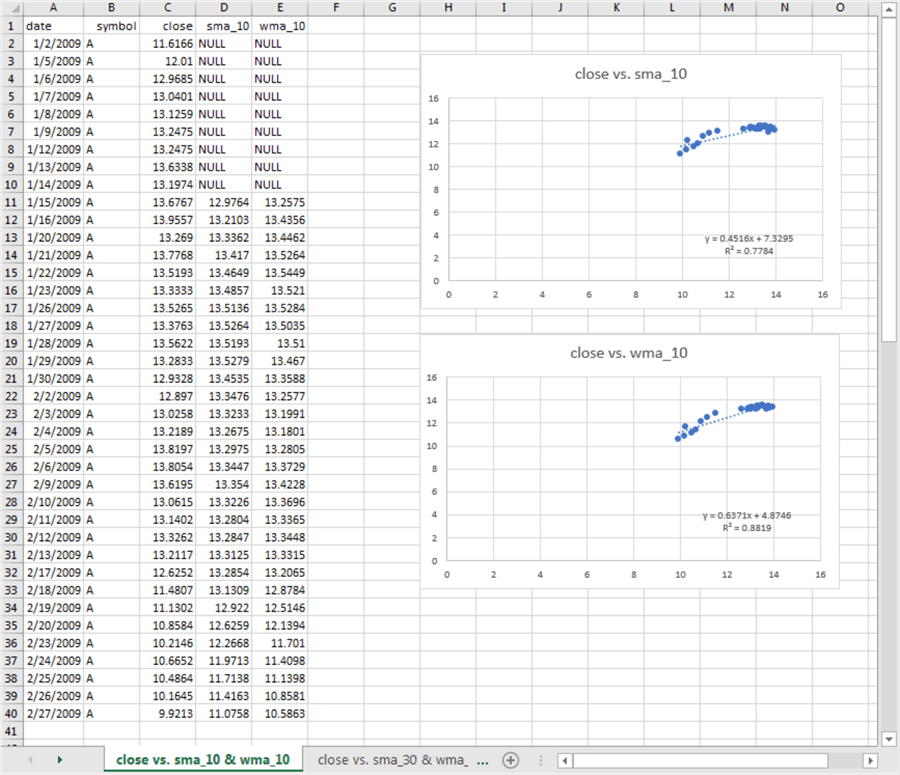
When focusing on the smoothing benefit of moving averages, you can ask the question: do you get the same degree of correspondence with underlying values for two different types of moving averages with the same period length? The first screen shot in this section shows the results from comparing a simple moving average with a period length of ten (sma_10) to a ten-period linear weighted moving average (wma_10).
- Both sets of moving averages are based on the first thirty-nine close prices for a stock represented by the symbol A. These data points start on 1/2/2009 and extend through 2/27/2009.
- Both sets of moving averages (sma_10 and wma_10) have null values for the first nine trading days. This is because the computational techniques for both simple moving averages and linear weighted moving averages are undefined until there are enough values to fill all the data points for one full period length. This outcome is not met until the date 1/15/2009, which is the tenth trading date starting from 1/2/2009.
- To the right of the data columns are two scatter diagrams for the comparison of the actual close prices to sma_10 and wma_10 values. The scatter diagrams are for data points starting on 1/15/2009 and running through 2/27/2009.
- As you can see, both sets of moving averages include values that approximately match the underlying close values. However, the coefficient of determination is greater when comparing wma_10 values to actual close prices (.8819) than when comparing sma_10 values to actual close prices (.7714).
Another interesting comparison is for sma_10 moving averages versus actual close prices relative to exponential weighted moving averages (ewma_10) versus actual close prices. The following screen shows selective results for ewma_10 values relative to actual close prices versus sma_10 values relative to actual close prices. There are three charts comparing actual close prices to moving average values.
- The top chart is for the comparison of the sma_10 values to actual close prices. This chart is also available from the preceding screen shot. The chart is duplicated here for easy comparison purposes. Recall that the data points and fit statistics are for dates from 1/15/2009 through 2/27/2009.
- The second chart is for the comparison of the ewma_10 values to the actual close prices. This chart is presented in this tip in the screen shot below. The date range is also from 1/15/2009 through 2/27/2009. The coefficient of determination for the second chart (.8696) is obviously greater than for the first chart (.7784). Therefore, for this sample of data, it is safe to conclude that ewma_10 values more closely match actual close prices than sma_10 values.
- However, the ewma_10 values have a slightly lower coefficient of determination with the actual close prices (.8696) than wma_10 values have with actual close prices (.8819). In interpreting these different outcomes, you need to understand that the wma_10 values can vary with the weights that are designated for the ten underlying values. It is also possible for ewma_10 values to change – for example, if you were to change the exponential smoothing constant. In my experience, exponential smoothing constants do not change when working with financial data, but linear weights for wma_10 values are more likely to change just because there is no widely accepted standard on what weight values should be. This may be one reason that exponential weighted moving averages are more commonly used than linear weighted moving averages.
- Exponential moving averages have another special feature. This is that exponential weighted moving averages can be defined as soon as the second value in the underlying series, but weighted moving averages are not available until the number of periods in the period length. This is especially relevant if you are using a long period length, such as a two-hundred-day moving average. For the sample of data in the screen shot below, the coefficient of determination for ewma_10 values starting on 1/5/2009 is .6451. While this value is not exceedingly large, the ewma_10 values are available over a considerably larger range of dates than for sma_10 and wma_10 values.

Next Steps
- The T-SQL scripts and worksheets for data displays and analyses are available in this tip’s download file. If you want to test the code with the data used for demonstrations in this tip, then you will also need to run scripts from here Collecting Time Series Data for Stock Market with SQL Server and Time Series Data Fact and Dimension Tables for SQL Server.
- Try out the code examples for this tip. For example, compute coefficients of determination for moving averages based on thirty periods instead of just ten periods. You can perform this with data provided in the download file for this tip.
- Another variation that you can try is to use your own data. Confirm the moving averages based on ten-period lengths are generally close to the underlying values. This period length will be the easiest to verify by manual computation. Next, compute moving averages based on thirty-period lengths for your data. In general, a ten-period moving average should more closely match underlying values than a thirty-period moving average.

Rick Dobson is a SQL Server professional with decades of T-SQL experience that includes authoring books, running a national seminar practice, working for businesses on finance and healthcare development projects, and serving as a regular contributor to MSSQLTips.com. He has been a practicing Python developer for more than the past half decade – with a special emphasis for data visualization and ETL tasks with JSON and CSV files. His most recent professional passions include financial time series data and analyses, AI models, and statistics. If you are interested in growing your skills in any of these areas especially as they relate to financial securities, consider visiting his blog at https://securitytradinganalytics.blogspot.com/2023/12/.
- MSSQLTips Awards: Leadership (200+ tips) – 2025 | Author of the Year Contender – 2017-2024


