How to Compute Simple Moving Averages with Time Series Data in SQL Server

By: Rick Dobson | Comments | Related: > TSQL

Problem

Demonstrate techniques for use of SQL Server Windows functions to compute simple moving averages. More specifically, highlight the use of the Windows aggregate avg function for computing simple moving averages for one entity at a time or concurrently for multiple entities. Present a framework that illustrates how to assess if simple moving averages can project accurately future time series values.

Solution

A prior tip, Time Series Data Fact and Dimension Tables for SQL Server, illustrated how to populate a data warehouse with time series data. One reason for populating a warehouse with time series data is to verify if past trends, as indicated by simple moving averages, can project future time series values. This kind of modeling activity relies on the notion that prior time series values point to future time series values.

This tip introduces you to the basics of computing simple moving averages for time series values in a data warehouse.

This tip's first example computes simple moving averages for two different period lengths for a single entity. MSSQLTips.com offers a tutorial on Windows functions with a section on statistical aggregate functions, such as avg. This tip applies the background from that tutorial section for computing simple moving averages.
Next, a more advanced example shows how to compute simple moving averages for four different period lengths over a set of entities from a data warehouse.
The tip concludes with a T-SQL demonstration for projecting future time series values based on historical time series trends for a selection of entities from a data warehouse.

Compute Simple Moving Averages for Two Different Periods for a Single Entity

A simple moving average is the arithmetic average of time series values for a window of periods anchored by the current period as the final period in the window. For example, a ten-period moving average is the average of the last ten periods, including the current one. The simple moving average window changes for successive new periods in a time series because the first period from the prior simple moving average window drops, and the current period becomes a new anchor. This prior tip includes a lengthier, but more introductory presentation, of simple moving averages.

You can have multiple moving averages with different lengths for the same time series data. For example, the select statement in the following script shows how to compute simple moving averages with ten-period and thirty-period lengths. All the simple moving average values are for the close prices of a stock represented by a symbol of A. The source data are from a table named yahoo_prices_valid_vols_only in the dbo schema of the for_csv_from_python database. This table was initially populated as the fact table in a data warehouse for historical stock price and volume data.

The yahoo_prices_valid_vols_only table has one close price per date.
Each date value corresponds to a trading date during which the NASDAQ, NYSE, and AMEX stock exchanges are open. These trading dates exclude weekend calendar days as well as about ten holidays per year when the exchanges are not open for trading.
The code attempts to compute simple moving averages for the first thirty-nine trading dates in the yahoo_prices_valid_vols_only table. The top clause specifies this constraint.
There is a separate case statement for computing the simple moving average (sma) for each of the two period lengths.
- Simple moving averages are not valid until enough periods pass to populate all the elements of a simple moving average window. The when clause condition within each case statement routes control to either
  - A Windows aggregate avg function for computing the simple moving average for a date
  - A null value when the function window has less than the minimum required number of trading dates for computing a simple moving average. This is
    - Nine trading dates before the current date for the ten-period moving average
    - Twenty-nine trading dates before the current date for the thirty-period moving average
- The Windows aggregate avg function within each case statement can compute the simple moving average for a period when there are enough periods to compute the value.
  - The avg function applies to the close values within the simple moving average window.
  - The over clause within the Windows aggregate avg function specifies the Windows range from
    - Nine trading dates before the current trading date through to the current trading date for the ten-period simple moving average
    - Twenty-nine trading dates before the current trading date through to the current trading date for the thirty-period simple moving average
The use statement preceding the select statement as well as the from and where clauses within the select statement combine to designate the range of values over which attempts are made to compute the simple moving average values.
- The use statement designates the database with your time series data. This tip relies on data from the for_csv_from_python database.
- The from clause specifies the table name and the schema name in which the table of time series values resides.
- The where clause restricts attempts to compute simple moving averages for close prices of a stock represented by the symbol A.

use for_csv_from_python
go
 
-- adaptation from https://www.mssqltips.com/sqlservertip/5248/mining-time-series-data-by-calculating-moving-averages-with-tsql-code-in-sql-server/
-- for first 39 time periods of ten-period and thirty-period moving averages for A
-- time series close values from [dbo].[yahoo_prices_valid_vols_only]
 
select 
 top 39
 [date]
,[symbol]
,[close]
-- for ten-period moving average
,
case
   when row_number() OVER(ORDER BY [Date]) > 9
      then avg([Close]) OVER(ORDER BY [Date] ROWS BETWEEN 9 PRECEDING AND CURRENT ROW)
   else null
end case_sma_10
-- for thirty-period moving average
,
case
   when row_number() over(order by [date]) > 29
      then avg([close]) over(order by [date] rows between 29 preceding and current row)
   else null
end case_sma_30
from [dbo].[yahoo_prices_valid_vols_only]
where symbol = 'A'

Here are the thirty-nine rows of output from the preceding script.

The date column includes the first thirty-nine trading dates from the yahoo_prices_valid_vols_only table.
The symbol column values correspond to the specified condition in the where clause from the select statement.
The close column values are the close prices over which attempts are made to compute simple moving averages.
The case_sma_10 column values are the results from the first case statement to compute ten-period simple moving average values.
- The first nine values are NULL because a ten-period simple moving average is not defined until there are at least ten time series values available.
- The first non-null ten-period simple moving average has a value of 12.9764. This is the arithmetic average of the close prices from 2009-01-02 through 2009-01-15.
- The second non-null ten-period simple moving average has a value of 13.2103, which is the arithmetic average of the close prices from 2009-01-05 through 2009-01-16. Notice that the date range for the second simple moving average moves the window down one date in the range of trading dates.
The case_sma_30 column values are the results from the second case statement to compute thirty-period simple moving averages.
- The first twenty-nine rows in this column are NULL because a thirty-period moving average Is not defined until there are thirty values over which to compute the moving average.
- The first non-null thirty-period simple moving average has a value of 13.2475. This is the arithmetic average of the close prices from 2009-01-02 through 2009-02-13.
- Each successive non-null thirty-period simple moving average is for the range of close prices corresponding to a window ending with the current trading date that is one trading date later than the preceding moving average and starting with a trading date that is one trading date later than the window for the preceding moving average.

Compute Simple Moving Averages for Four Different Periods for Multiple Entities

While it can be of value to compute simple moving averages for a single entity, database professionals will more likely be computing simple moving averages when there are many different entities. Furthermore, it is sometimes the case that there will be a need to compute simple moving averages for more than two period lengths. This section demonstrates computational techniques for these cases by building on the code from the preceding section and by using the same source data as the preceding section with different filters.

Before presenting the code and results for computing simple moving averages with four different periods for multiple entities, it may be useful to review some basic data mining queries for the source data. As mentioned, the sample time series data for this tip resides in the yahoo_prices_valid_vols_only table.

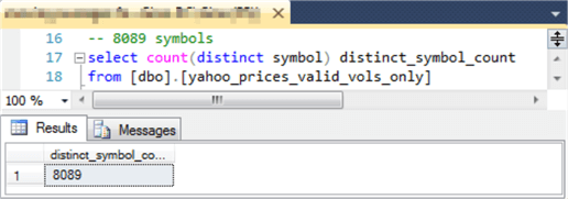
The following query and its results set shows there are 8089 distinct symbols in the yahoo_prices_valid_vols_only table.

Each symbol in the yahoo_prices_valid_vols_only table has time series data values for a certain range of trading dates. The time series values for the symbols were collected from Yahoo Finance starting with the first trading date in 2009 through October 7, 2019. However, not all symbols were trading as of the first trading date in 2009, and some symbols were dropped from the NASDAQ, NYSE, and AMEX exchanges prior to October 7, 2019. The following query and results set shows the maximum number of distinct trading dates (2709) for time series data in the yahoo_prices_valid_vols_only table.

The following query and results set shows how to count the number of symbols with time series values for each distinct trading date in the yahoo_prices_valid_vols_only table. The query groups the table rows by symbol and constrains the output to just those symbols with a count of rows equal to 2709, which is the maximum number of distinct trading dates in the table. The following screen shot confirms there are 2614 symbols having a row for each possible trading date.

Now that you have a basic feel for the extent of the time series values in the yahoo_prices_valid_vols_only table, this tip returns its focus to the T-SQL code for computing simple moving averages with multiple period lengths for multiple symbols. The sample code below computes simple moving averages with lengths of ten, thirty, fifty, and two hundred periods for three symbols – A, AA, AAPL. While this code is generally like the code in the preceding section for a couple of simple moving averages for a single symbol, the following code exposes some critical techniques for efficiently processing more than one symbol and simple moving averages for more than two period lengths.

There is a separate case statement for each period length.
- The name for the case statement computing a ten-period length is case_sma_10.
- Similarly, the names of the case statements for the other period lengths are case_sma_30, case_sma_50, and case_sma_200.
The where clause specifies a list of distinct symbol values for which simple moving averages are computed.
The over clause in the when condition expression is updated to include a "partition by [symbol]" phrase. This phrase allows the Windows function to freshly compute the simple moving average with a period length for each symbol in the where clause.

-- demonstration code for ten-period, thirty-period, fifty-period, and two-hundred-period 
-- simple moving averages for three symbols (A, AA, AAPL)
select 
 [date]
,[symbol]
,[close]
-- for ten-period moving average
,
case
   when row_number() over(partition by [symbol] order by symbol,[date]) > 9
      then avg([Close]) over(order by symbol,[date] rows between 9 preceding and current row)
   else null
end case_sma_10
-- for thirty-period moving average
,
case
   when row_number() over(partition by [symbol] order by symbol,[date]) > 29
      then avg([close]) over(order by symbol,[date] rows between 29 preceding and current row)
   else null
end case_sma_30
-- for fifty-period moving average
,
case
   when row_number() over(partition by [symbol] order by symbol,[date]) > 49
      then avg([close]) over(order by symbol,[date] rows between 49 preceding and current row)
   else null
end case_sma_50
-- for two-hundred-period moving average
,
case
   when row_number() over(partition by [symbol] order by symbol,[date]) > 199
      then avg([close]) over(order by symbol,[date] rows between 199 preceding and current row)
   else null
end case_sma_200
from [dbo].[yahoo_prices_valid_vols_only]
where symbol in('A','AA', 'AAPL')

Here are some selected excerpts from the preceding script.

The first thirty-five rows from the results set appear in the following screen shot.

The rows progress from the first trading date (2009-01-02) through the thirty-fifth trading date (2009-02-23) for the A symbol.
This screen shot allows you to view the beginning of the ten-period simple moving average (case_sma_10) and thirty-period simple moving average (case_sma_30) for the A symbol.
You can also see the columns for the fifty-period and two-hundred-period simple moving averages (case_sma_50 and case_sma_200, respectively), but these columns have null values in the screen shot because the rows extend only to the thirty-fifth row. The simple moving averages with these two period lengths do not start until the fiftieth and two-hundredth rows, respectively.

The next screen shot shows rows 195 through 205 in the results set.

Row 200, which is highlighted, shows the first two-hundred-period simple moving average value in the case_sma_200 column.
The case_sma_50 column shows fifty-period simple moving average non-null values in rows 195 through row 205. Non-null values for the case_sma_50 column initially appear starting in row 50.
All the results in this screen shot and preceding one are for the A symbol.

The next screen shot shows a transition for results from the A symbol to results for the AA symbol.

Row 2709 is the first highlighted row. This is the last row of results for the A symbol. The date value for the row is 2019-10-07.
Rows 2710 through 2718 show the first nine rows for the AA symbol with no computed simple moving averages.
Rows 2719 through 2723 shows the first five ten-period simple moving average values for the AA symbol with a value different than NULL.

The last screen shot in this section is for the final five rows in the results set from the preceding script.

These rows are all for the AAPL symbol.
The very last row has a row number of 8127. Because there are 2709 rows for each of the three symbols used in this section, the row number of 8127 confirms the right number of simple moving averages were computed by the preceding script (3 times 2709).

Using Simple Moving Average Differences to Predict Future Time Series Values

At any given point in time, the relationships between simple moving averages of different period lengths can convey a sense of the trend of the underlying time series values. If simple moving averages with shorter periods have larger values than simple moving averages with longer periods, then the trend of time series values is increasing. This is because more recent time series values have a larger average than time series values that are less recent.

Within the context of this tip, if the ten-period simple moving average is greater than the thirty-period simple moving average, and the thirty-period moving average is greater than the fifty-period simple moving average, and the fifty-period simple moving average is greater than the two-hundred-period simple moving average, then the underlying time series values are increasing from two hundred days ago through ten days ago. In other words, the underlying time series values are moving up. Furthermore, the larger the summed sma differences, the larger the trend.

We can ask the question, if the trend of underlying prices is moving up will they continue to move up through the next five days – or whatever other period for which you care to test? The notion that trends for prior time series values can predict future time series values is a common one for time series analysis. Simple moving averages like those from either of the preceding two sections can help to assess if trends for prior time series values help to predict future time series values. This section gives an example of one approach for answering this kind of question.

The following screen shot shows an Excel worksheet into which values of ten-period, thirty-period, fifty-period, and two-hundred-period simple moving averages were copied from the Results pane of SQL Server Management Studio for the MSFT symbol in calendar year 2010.

The copied values appear in columns A through G.
Columns I through K are hidden to improve the readability of the worksheet. These hidden columns contain expressions that compute, respectively, the differences of the ten-period less the thirty-period, the thirty-period less the fifty-period, and the fifty-period less the two-hundred-period simple moving averages.
The sum of the differences from column I through K show in column L.
Column M displays the close price for five trading days after the current trading date. For example, the close_lead5 cell value in row 2 matches the close cell value in row 7.
The graph to the right shows the regression of the close_lead5 column values on the estimated close_lead5 values.
- The estimated close_lead5 values appears as a straight line depicted by small dots with the summed sma differences from column L and their matching actual close_lead5 values from column M appearing as larger dots around the line.
- The equation for calculating estimated close_lead5 values appears below line on its right side; this equation is derived through built-in Excel features.
  - The slope has the value 0.6464. Therefore, the estimated close_lead5 value grows around .64 points for each one-point increase in the summed sma differences.
  - The intercept has the value 27.08, which means the estimated close_lead5 value equals 27.08 when the summed sma differences equals zero.
The goodness of fit appears below the regression equation.
- The goodness is denoted by a coefficient of determination value (R²) whose value can vary between 0 for no fit at all to 1 for a perfect fit.
- The R² value of .7573 means that about seventy-five percent of the future closing price values five trading days later are explained by the sum of the sma differences from today.

A worksheet with the same layout was created for the MSFT symbol simple moving average and close prices during 2017. You can see in the preceding screen shot the tab for MSFT data in 2017 to the right of the tab for MSFT data in 2010.

Additionally, other worksheets with summed sma differences and leading close prices were developed for these other nine symbols: GOOGL, AMZN, AMD, AAPL, FEZ, EPP, CLNE, BHP, and ALB. The preceding screen shot shows two worksheet tabs for GOOGL and one worksheet tab for AMZN. Each symbol, whether in the screen shot or not, had its future close prices regressed separately against its summed sma differences for two different years. Therefore, data were processed for twenty different combinations of symbol and year. The summary of the results appears below. There are three key points to note.

The slope across the twenty regressions for ten symbols for each of two different years was always positive. This confirms that for the ten symbols across two different years there was always a positive trend between the sum of sma differences today and the close price five trading days later.
The coefficient of determination (R²) was typically well above zero for all combinations of symbol and year, which indicates that changes in the sum of the sma differences were consistently correlated with changes in close prices five trading days later.
On average across the twenty regressions for symbol and year, the sum of sma differences accounted for about sixty percent of the variation in the close prices five trading days later.

Next Steps

The T-SQL scripts and worksheet analyses are in this tip's download file.
Try out the code examples for this tip. For example, vary a parameter for the code samples as well as for the example in the Excel workbook file.
If you want to test the code with the data used for demonstrations in this tip, then you will also need to run scripts from here Collecting Time Series Data for Stock Market with SQL Server and here Time Series Data Fact and Dimension Tables for SQL Server.

About the author

Rick Dobson is an author and an individual trader. He is also a SQL Server professional with decades of T-SQL experience that includes authoring books, running a national seminar practice, working for businesses on finance and healthcare development projects, and serving as a regular contributor to MSSQLTips.com. He has been growing his Python skills for more than the past half decade -- especially for data visualization and ETL tasks with JSON and CSV files. His most recent professional passions include financial time series data and analyses, AI models, and statistics. He believes the proper application of these skills can help traders and investors to make more profitable decisions.

This author pledges the content of this article is based on professional experience and not AI generated.

View all my tips