Spark Data Exploration with Azure Synapse

By: Fikrat Azizov | Comments | Related: > Azure Synapse Analytics

Problem

Azure Synapse Analytics comes with several exciting data exploration features. In the Explore your SQL databases with Azure Synapse Analytics we investigated Azure Synapse Analytics' data exploration features related to the SQL pools.

The Spark support in Azure Synapse Analytics brings a great extension over its existing SQL capabilities. Users can use Python, Scala, and .Net languages, to explore and transform the data residing in Synapse and Spark tables, as well as in the storage locations. This also made possible performing wide variety of Data Science tasks, using this platform.

In this tip we are going to learn how to use Spark notebooks to explore data in SQL and Spark databases as well as in the storage account.

Solution

Create a Spark Pool

As you may have guessed already, we will need to add a Spark pool, to be able to benefit from Spark features.

Let us add a Spark pool, using Manage tab, the similar way we did for SQL pools. Provide the name, node size and number of the nodes in the pool:

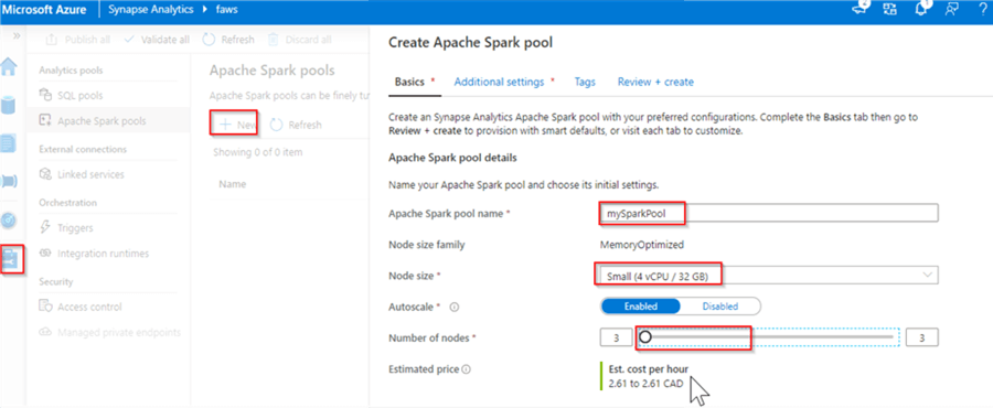
Figure 1

Next, switch to Additional settings tab and review the following settings:

Number of minutes idle - This parameter determines how long will Spark wait until it shuts down the cluster if it has no active jobs.
Apache Spark - The Spark version (currently only the Spark 2.4 is available)

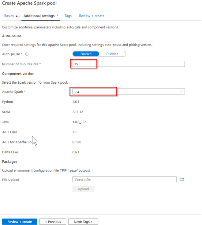
Figure 2

Once the pool provisioned, we can leverage it to execute our Spark notebooks.

Exploring SQL to Spark Integration

One of the great advantages of Azure Synapse Analytics is its ability to provide a seamless integration between its components.

I think the easiest way to learn the integration between SQL and Spark components of the Synapse Analytics is to generate a table-read code from the object explorer. To do that, let us navigate to the Data tab, select the DimProduct table, and click the 'Actions/New notebook/Load to DataFrame' command, as follows:

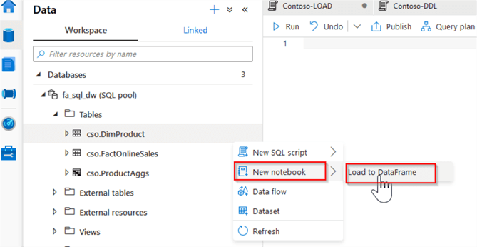
Figure 3

This creates a Scala notebook, with the following code:

Val df = spark.read.sqlanalytics("fa_sql_dw.cso.DimProduct")
// df.show(10)

Notice that we did not need to supply any connection strings. You may also have noticed that the execution context automatically changes to the Spark pool, and Scala gets selected as a programming language, when we generate a table read code. We can change the notebook's default language to PySpark, Spark SQL and .Net if needed, however keep in mind that SQL DW read/write functions like in the sample above, are only available in Scala language at this point.

Here is my screenshot:

Figure 4

Let us slightly modify the above code, so that it displays the results in a formatted way, as follows:

val df = spark.read.sqlanalytics("fa_sql_dw.cso.DimProduct")
display(df)

You can run this code either by opening a command palette at the top right corner of the cell and selecting the Run cell command, or by entering a combination of Ctrl+Enter keys. Here is the output:

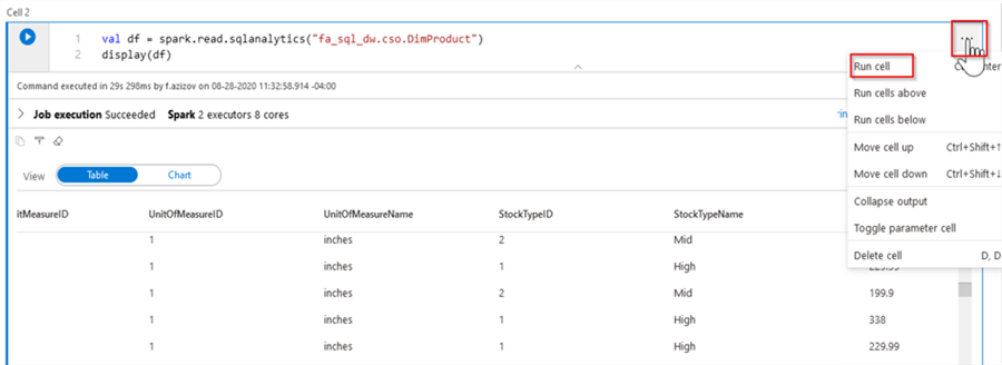
Figure 5

Next, let us add a new cell, using the Add code button at the bottom of the current cell, then add the following simple aggregations code and run it:

val dfAgg=df.groupBy("ClassName").count()
display(dfAgg)

We can monitor the job's progress, by expanding little arrow at the bottom left corner of the cell:

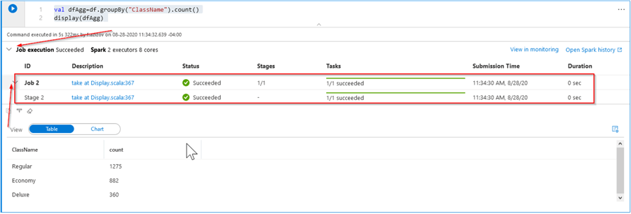
Figure 6

Next, let us write the dfAgg data frame back into the SQL database, using the following code.

dfAgg.write.sqlanalytics("fa_sql_dw.cso.ProductAggs", Constants.INTERNAL)

Once the script ran, we can refresh the table list in the object explorer and ensure that the new table has been added:

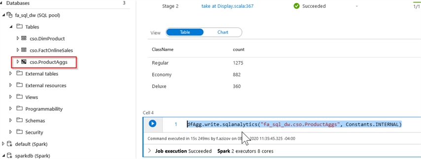
Figure 7

Next, let us create a Spark database and write the dfAff data frame there as a table, using the following code:

spark.sql("CREATE DATABASE IF NOT EXISTS SparkDb")
dfAgg.write.mode("overwrite").saveAsTable("SparkDb.ProductAggs")

Now we can navigate to the Data tab, refresh the database list, and confirm that we have got a newly created sparkdb database:

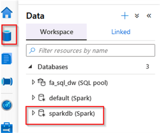
Figure 8

Finally, let me demonstrate how we can read the content of the Spark table, using only Spark SQL commands. There are couple of ways to use Spark SQL commands within the Synapse notebooks – you can either select Spark SQL as a default language for the notebook from the top menu, or you can use SQL magic symbol (%%), to indicate that only this cell needs to be run with SQL syntax, as follows:

%%sql
Select * from SparkDb.ProductAggs

Exploring the Spark to Storage Integration

We can automatically generate a code to read the storage data the same way we did for SQL tables.

Let us navigate to the Data pane and open the content of the default container within the default storage account. Next, select the CSV file we created earlier and create a notebook to read it, by opening right-click context menu and selecting the New notebook command, as follows:

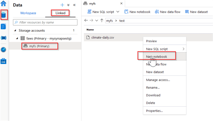
Figure 9

Here is the script generated inside the PySpark notebook:

%%pyspark
data_path = spark.read.load('abfss://[email protected]/test/climate-daily.csv', format='csv'
## If header exists uncomment line below
##, header=True
)
display(data_path.limit(10))

Because our CSV file has column headers, I will uncomment the header related line and run the cell, as follows:

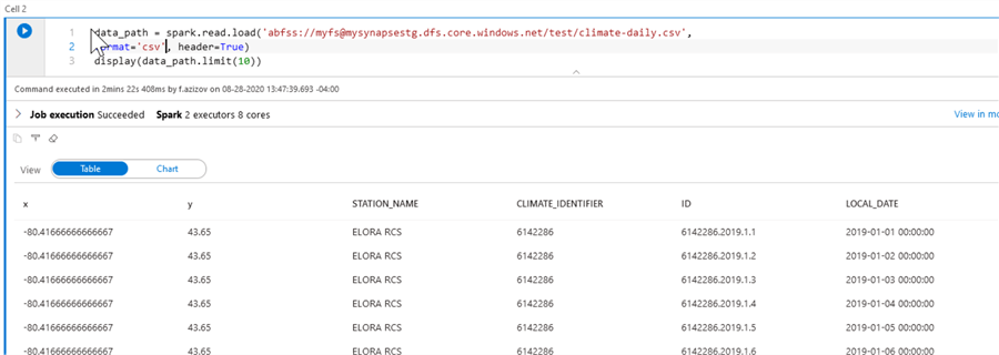
Figure 10

Next Steps

About the author

Fikrat Azizov has been working with SQL Server since 2002 and has earned two MCSE certifications. He’s currently working as a Solutions Architect at Slalom Canada.

This author pledges the content of this article is based on professional experience and not AI generated.

View all my tips

Explore Spark databases with Azure Synapse Analytics