Problem
The Spark engine supports several different file formats. Therefore, it is important to understand the pros and cons of each file type. Additionally, Hive tables can be classified as managed and unmanaged. Which one is best for your organization?
Solution
A basic understanding of Spark clusters and partitioning is required to reduce the processing time of Spark queries. Today, we will look at the two airline flight datasets included with each Azure Databricks distribution. We want to engineer a set of tables for use in future Spark MSSQLTips.com articles. During this process, we will review file formats and Hive table types.
Business Problem
Create Hive tables for airline performance data, airplane description data, and airport location data. We will explore different Spark file and Hive table formats during this demonstration. Ultimately, we will better understand file formats and table types.
User Defined Functions
Like most third-generation languages, Python supports the declaration of functions. Let’s define some functions to help with files and folders. The user function named delete_dir is shown below. This function will remove the contents of a given directory using recursive calls to the dbutils library.
#
# delete_dir - remove all content in given directory
#

def delete_dir(dirname):
  try:
    # get list of files + directories
    files = dbutils.fs.ls(dirname)

    # for each object
    for f in files:

      # recursive call if object is a directory
      if f.isDir():
        delete_dir(f.path)

      # remove file or dir
      dbutils.fs.rm(f.path, recurse=True)

    # remove top most dir
    dbutils.fs.rm(dirname, recurse=True)
  except:
   pass
The different file formats supported by Spark have varying levels of compression. Therefore, getting the number of files and total bytes in a given directory is interesting. The user-defined function named get_file_info uses a similar recursive algorithm to traverse the folder structure. Note: A Python list is used to keep track of the size of the files and the number of files in a given directory. I could have used two variables, but I wanted to teach you, the reader, about data structures in Python. Finally, the function results are returned as a Python dictionary object.
#
# get_file_info - return file cnt + size in gb
#

def get_file_info(dirname):

  # variables
  lst_vars = [0, 0]

  # get array of files / dirs
  files = dbutils.fs.ls(dirname)

  # for each object
  for f in files:

    # object = dir
    if f.isDir():

      # recursive function call
      r = get_file_info(f.path)

      # save size / number
      lst_vars[0] += r['size']
      lst_vars[1] += r['number']

    # object <> dir, save size / number
    lst_vars[0] += f.size
    lst_vars[1] += 1

  # return data
  return {'size': lst_vars[0], 'number': lst_vars[1]}
Since many of the data files we work with are large, we want a function to transform the file size dictionary element from bytes into gigabytes. Why did I not do this calculation in the previous function? There would be rounding errors since we would perform division for each subdirectory.
#
# update_file_dict– update dictionary
#

def update_file_dict(type_dict, dir_dict):

  # get size in bytes, convert the size to gigabytes
  old = dir_dict.get("size")
  new = (old / 1024 / 1024 / 1024)

  # update size value, add type element
  dir_dict.update({'size': new})
  dir_dict.update(type_dict)

  # return the results
  return dir_dict
The above function, called update_file_dict,updates the size from bytes to gigabytes. Additionally, it will add a new element to the dictionary for the file type. We will use an array of dictionaries to keep the results of our file type exploration in the future.
Let’s try out these new functions. The Python code below removes the simple data lake from the DBFS local storage using the delete_dir function. This code assumes the directory exists and has content.
# remove existing directory
delete_dir("/lake2022")
If we search the sample datasets installed with Azure Databricks, we find the asa directory with airline information. This information is focused on both departure and arrival delays. Information such as airplane tail number and airport location code is also included. The image below shows 22 CSV files for the years 1987 to 2008. The magic file system command (%fs) was used with the ls command to produce a list of files in the fully qualified path.
![Spark File + Hive Tables - list [asa] airline files.](/wp-content/images-tips/7492_working-with-spark-files-and-hive-tables.001.png)
The Python code below calls both the get_file_info and update_file_dict functions. We can see that the 22 files in the asa directory use 11.20 gigabytes of file space.
![Spark File + Hive Tables - collect [asa] airline files - total size](/wp-content/images-tips/7492_working-with-spark-files-and-hive-tables.002.png)
Databricks Architecture
Why are file storage space and file partitioning important?
The image below was taken from an MSDN article on Azure Databricks architecture. As a big data developer, you are familiar with the control pane. For instance, to create new notebooks, one must have an active cluster. Each time you run a cell during debugging, you send a request to the data plane. The computing power of the cluster consists of n worker nodes and 1 executor node. In reality, all nodes in the cluster are virtual machines running a version of LINUX. The most important part of the diagram is the get and put requests to the Databricks File System (DBFS).
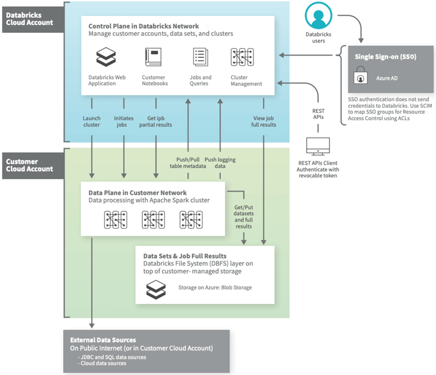
This layer is an abstraction to the given cloud vendor storage. Databricks is a multi-cloud product that runs on Microsoft Azure, Amazon Web Services (AWS), and Google Cloud Platform (GCP). We know that storage is a lot slower than the memory used by the Spark cluster. Therefore, the faster we can load into memory, the faster our jobs and/or queries run. A file format that supports both compression and partitioning is optimal for Spark.
In a nutshell, both the file size and file partition affect the execution of Spark programs. There is much more to this tuning topic than what can be covered today.
Simple Data Lake
To compare different file formats, we need to create a simple folder structure to contain reformatted airline data. The magic command for a LINUX Bourne Shell (%sh) allows the developer to use the mkdir command to create directories, as seen in the code block below.
%sh
mkdir /dbfs/lake2022
mkdir /dbfs/lake2022/bronze
I am going to skip to the end of the article to show you what file types we are going to experiment with. The ls command lists the contents of a given directory. The code block below creates a directories list in the bronze zone.
%sh
ls /dbfs/lake2022/bronze
The image below shows six file formats that will be reviewed in this article.

Sample Datasets
To demonstrate, four different sample datasets have been identified below. The files reside in two different sub-directories in the Databricks File System. Using the following code, let’s load the information as temporary views from the CSV files. Then, in the next section, we can explore the rows of data, specifically data quality, using Spark SQL.
Dataset 1: tmp_airline_data
#
#  2 - Read airline (performance) data
#

# file location
path = "/databricks-datasets/asa/airlines/*.csv"

# make dataframe
df1 = spark.read.format("csv").option("inferSchema", "true").option("header", "true").option("sep", ",").load(path)

# make temp hive view
df1.createOrReplaceTempView("tmp_airline_data")

# show schema
df1.printSchema()
Dataset 2: tmp_plane_data
#
#  3 - Read plane data
#

# file location
path = "/databricks-datasets/asa/planes/*.csv"

# make dataframe
df2 = spark.read.format("csv").option("inferSchema", "true").option("header", "true").option("sep", ",").load(path)

# make temp hive view
df2.createOrReplaceTempView("tmp_plane_data")

# show schema
df2.printSchema()
Dataset 3: tmp_flight_delays
#
#  4 - Read departure + delay data
#

# file location
path = "/databricks-datasets/flights/departuredelays.csv"

# make dataframe
df0 = spark.read.format("csv").option("inferSchema", "true").option("header", "true").option("sep", ",").load(path)

# make temp hive view
df0.createOrReplaceTempView("tmp_flight_delays")

# show schema
df0.printSchema()
Dataset 4: tmp_airport_codes
#
#  5 - Read airport codes
#

# file location
path = "/databricks-datasets/flights/airport-codes-na.txt"

# make dataframe
df3 = spark.read.format("csv").option("inferSchema", "true").option("header", "true").option("sep", "\t").load(path)

# make temp hive view
df3.createOrReplaceTempView("tmp_airport_codes")

# show schema
df3.printSchema()
Exploring Datasets
The queries to return five rows of data from the temporary views are simplistic. Therefore, I will not include them during our discussion. I suggest you look at the final enclosed notebook at the end of the article for complete details.
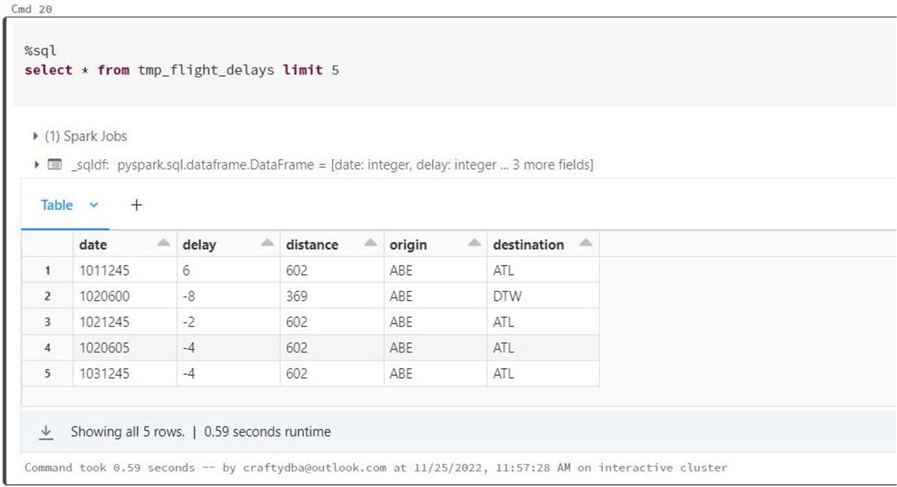
Flight Delays Dataset
The image below shows the flight delays dataset. This dataset has most of the fields removed from the source, and the date is stored in a format that is not recognized. That said, I will not promote this data as a Hive table, and it will be discarded as an invalid dataset.
Airlines Dataset
The airlines dataset contains a lot of fields. The image below shows the fields I thought were most important. A simple calculation was used to turn the year and month into a 6-digit hash key called FltHash. This key can be used to partition the data in the future.

Plane Data Dataset
For a given tail number in the airline dataset, we can retrieve detailed information about the airplane. There is some null data in the source file for some rows. A business analyst might be tasked with cleaning up the file in the real world. The image below randomly shows five records from the temporary view.

Airport Codes Dataset
Both origin and destination airports are assigned codes in the airline dataset. The airport dataset will allow the end user to decode this information into a physical location in the world. The image below shows that code ABR represents Aberdeen, South Dakota.

Examining the Data
The first step when exploring a new set of data files is to understand the number of records we are dealing with. The Spark SQL code below gets the record counts from all three temporary views.
%sql
-- Get record counts
select 'codes' as label, count(*) as total from tmp_airport_codes
union
select 'airports' as label, count(*) as total from tmp_airline_data
union
select 'planes' as label, count(*) as total from tmp_plane_data
We can see we have hundreds of airport codes and thousands of airplanes. This is considered small data. However, we have over 123.53 million recorded flights in the last 22 years. This might be regarded as medium size data.

Since the airlines view can be considered the main table, the airport and/or airplane views can be considered lookup tables. It would be nice to know if we have missing data in our lookups. The Spark Query below retrieves a count of how many issues we have with airport codes.
%sql
-- Find unmatched airport codes
select count(*) as total
from tmp_airline_data as a
left join tmp_airport_codes as c1 on a.Origin = c1.IATA
left join tmp_airport_codes as c2 on a.Dest = c2.IATA
where c1.city is null or c2.city is null
We have 1.66 million records that do not have a valid airport code. In a future article, we will discuss obtaining missing data, such as airport codes from web pages. In short, this is not a really bad issue.

Upon grouping the tail numbers for the airline dataset, I noticed four planes’ tail numbers that can be considered unknown. In fact, we could update this data in the future to a consistent text value such as an ‘UNKNOWN’.
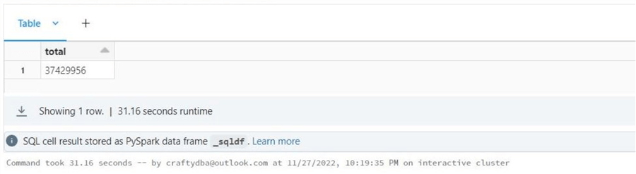
%sql
-- Bad tail numbers
select count(*) as total
from tmp_airline_data as a
where a.tailnum in ('NA','UNKNOWN','�NKNO�','null')
The image below shows that 37.42 million rows have unknown plane tail numbers, or about 30.29 percent of the records.
The last query is to find how many tail numbers that seem to be valid in the airline dataset (view) but do not exist in the airplane dataset (view). Execute the following query to obtain this information:
%sql
-- Find unmatched airport codes
select count(*) as total
from tmp_airline_data as a
left join tmp_plane_data as p on a.tailnum = p.tailnum
where a.tailnum not in ('NA','UNKNOWN','�NKNO�','null') and p.tailnum is null
The image below shows that 38.02 million rows have plane tail numbers that do not exist in our dimension table or about 30.77 percent of the records.

In a nutshell, we have an issue with the airport codes dataset. However, it affects only 1.34 percent of the airline records. On the other hand, the airplane data (tail number) is not filled out for 30.29 percent of the airline records. Nothing can be done to fix this missing data issue. Additionally, there is another 30.77 percent of the airline records with unmatched tail numbers in the airplane data set.
It is important to know your data before making decisions. For instance, it will be hard to answer which manufacturers have the most planes in the air when 61 percent of the data is missing.
Managed Hive Tables
The main difference between managed and unmanaged Hive tables is the location of the data. With managed tables, the data is located in the Hive repository. Also, a drop table statement on a managed table removes the data. At the same time, a drop table statement on an unmanaged table removes the metadata from the Hive catalog.
Let’s start our investigation by dropping and recreating a Hive database (schema) named sparktips. See the code below for details.
#
#  7A – re-create database
#

# drop database
sql_stmt = "DROP DATABASE IF EXISTS sparktips CASCADE;"
spark.sql(sql_stmt)

# create database
sql_stmt = "CREATE DATABASE sparktips;"
spark.sql(sql_stmt)
We want to reuse the formatted airline data from the Spark SQL Query below since it has a hash key defined. Therefore, it is prudent to save the results in a dataframe named df4for future use.
#
#  7B - format airline data in final dataframe
#

# create table
sql_stmt = """
  select
    Year * 100 + Month as FltHash,
    Year as FltYear,
    Month as FltMonth,
    DayOfMonth as FltDay,
    DepTime,
    ArrTime,
    FlightNum,
    TailNum,
    ActualElapsedTime as ElapsedTime,
    ArrDelay,
    DepDelay,
    Origin,
    Dest,
    Distance as FltDist
  from tmp_airline_data
"""

# grab data frame
df4 = spark.sql(sql_stmt)

# row count
print(df4.count())
The code below creates a table named mt_airline_data. The prefix mt stands for “managed table”, and umt represents “unmanaged tables”. Note: We used the “format” method to choose a delta file format and the “partitionby” method to slice up our data. See Databricks documentation for details on Delta Lake.
#
#  7C - Write airline data (managed hive table)
#

# drop managed table
sql_stmt = "DROP TABLE IF EXISTS sparktips.mt_airline_data"
spark.sql(sql_stmt)

# write as managed table
df4.write.format("delta").partitionBy("FltHash").saveAsTable("sparktips.mt_airline_data")
The describe table extended Spark SQL command displays the details of a given Hive table. At the top of the output is a list of fields and data types, while a list of properties, such as file location, is at the bottom.
%sql
describe table extended sparktips.mt_airline_data
The image below captures the bottom output from the command. We can see that the table type is MANAGED, the data is partitioned by the FLTHASH column, and the files are stored under the HIVE directory.

If we look at the directory structure in DBFS, we can see that the name of the sub-directories reflects the partitioning.

The following two cells in the notebook create managed tables for airplanes and airports. Since the data is small, we want to ensure that only one partition (file) is created. The code below creates the table named mt_airplane_data.
#
#  8 - Write airplane data (managed hive table)
#

# drop table
sql_stmt = "DROP TABLE IF EXISTS sparktips.mt_airplane_data"
spark.sql(sql_stmt)

# grab data frame
df5 = spark.sql("select * from tmp_plane_data")

# write as managed table
df5.repartition(1).write.format("delta").saveAsTable("sparktips.mt_airplane_data")
The code below creates the table named mt_airport_data.
#
#  9 - Write airport data (managed hive table)
#

# drop table
sql_stmt = "DROP TABLE IF EXISTS sparktips.mt_airport_data"
spark.sql(sql_stmt)

# grab data frame
df6 = spark.sql("select * from tmp_airport_codes")

# write as managed table
df6.repartition(1).write.format("delta").saveAsTable("sparktips.mt_airport_data")
In a nutshell, we have all three datasets saved as managed delta tables in the Hive catalog. These tables will be used in our future exploration of Spark SQL. In the next section, we will explore unmanaged tables with various file formats.
Various Partitioned File Formats
We are now at the point in which we can leverage the dictionary functions we created earlier. The code snippet below creates an empty list. We will be appending results to this list during our discovery process.
#
#  10 - Create array to hold results
#

# empty list
results = []
It is best practice to write code that can be restarted if a failure occurs. The code below uses the format and save methods of the dataframe to create a partitioned avro dataset under the corresponding sub-directory. If we run this code again, it will fail since the directory exists. Therefore, starting the coding block with a delete_dir function call makes our code restartable.
#
#  10A1 - Write airline data (arvro)
#

delete_dir("/lake2022/bronze/avro")
df4.write.format("avro").partitionBy("FltHash").save("/lake2022/bronze/avro")
The next section of code gets file information about the avro format and appends this data to the results list.
#
# 10A2 - get file list (avro)
#

info = update_file_dict({'type': 'avro'}, get_file_info("/lake2022/bronze/avro"))
results.append(info)
The same code is called repeatedly for each of the following file formats. The table below shows the file size versus file type exploration.
| File Type | File Count | Size (GB) |
|---|---|---|
| AVRO | 1310 | 2.56 |
| CSV | 1304 | 5.85 |
| DELTA | 542 | 0.96 |
| JSON | 1304 | 23.56 |
| ORC | 1304 | 1.17 |
| PARQUET | 1304 | 0.96 |
Both the delta and parquet file formats are the smallest in size. This makes sense since delta uses parquet files. The delta file will only increase in size if data manipulation language (DML) actions are performed, such as inserts, updates, and deletes. More to come about the delta file format in a future article.
Creating Hive Table Over Existing Files
Our next task is to create metadata in the Hive catalog for various file formats partitioned by the flight hash key. There are two Hive settings we need to enable for dynamic partitions:
%sql
set hive.exec.dynamic.partition=true
set hive.exec.dynamic.partition.mode=nonstrict
The following code will be repeated for each file format except for delta. We will discuss that separate use case at the end of the section.
There are three steps we need to perform:
- Drop the Hive table if it exists.
- Create an external table by specifying the schema and partitioning.
- Repair the Hive table using the MSCK command. This action rescans the directory for partitions that might have been added or deleted at the file system level.
%sql

--
--  Unmanaged avro hive table
--

-- Drop existing
DROP TABLE IF EXISTS sparktips.umt_avro_airline_data;

-- Create new
CREATE EXTERNAL TABLE sparktips.umt_avro_airline_data
(
  FltYear int,
  FltMonth int,
  FltDay int,
  DepTime string,
  ArrTime string,
  FlightNum int,
  TailNum string
)
USING AVRO
PARTITIONED BY (FltHash int)
LOCATION '/lake2022/bronze/avro';

-- Register partitions
MSCK REPAIR TABLE sparktips.umt_avro_airline_data;
Copy the code block, modify it for most file types, and execute it to register the files as Hive tables.
The only exception to this rule is the delta file format. The code below has only two steps:
- Drop the unmanaged table if it exists.
- Recreate the unmanaged delta table.
Because delta has transaction log files, it knows all about the schema and partitioning of the data. Thus, repairing the table is not needed.
%sql

--
--  Unmanaged delta hive table
--

-- Drop existing
DROP TABLE IF EXISTS sparktips.umt_delta_airline_data;

-- Create new
CREATE EXTERNAL TABLE sparktips.umt_delta_airline_data
USING DELTA
LOCATION '/lake2022/bronze/delta';
The image below shows the three managed and six unmanaged tables in the Hive database named sparktips. This is the culmination of all the work we did in this tip. Now we can execute a simple performance test on the published tables.

Simple Query Comparison
The whole purpose of this article is to look at different file formats and Hive table types. Is there a speed difference between one type and (over) another? We are going to look at three different queries and collect execution times.
Query 1
The first query below counts the records for a given year and month. We are going to include the temporary view named tmp_airline_data in our test. Please remember that this is a temporary view on top of the 22 files that have the data grouped by year.
%sql
select count(*) from sparktips.umt_avro_airline_data where flthash = 200001
The same output is generated for all queries, as seen below.

The table below shows the results of this testing effort. Using the partition key in any query seems to speed up the return of the results.
| File Type | Run Time (sec) |
|---|---|
| AVRO | 0.68 |
| CSV | 0.76 |
| DELTA | 0.56 |
| JSON | 0.99 |
| ORC | 1.18 |
| PARQUET | 0.30 |
| TEMP VIEW | 30.02 |
Query 2
The second query below aggregates the number of flights by tail number for a given year and month:
%sql
select FltHash, TailNum, count(*) as Total
from sparktips.umt_avro_airline_data
where flthash = 200001 and TailNum is not null
group by FltHash, TailNum
The same output is generated for all queries (see below) and only returns the first 1000 rows.

The table below shows the results of this testing effort.
| File Type | Run Time (sec) |
|---|---|
| AVRO | 1.55 |
| CSV | 1.58 |
| DELTA | 4.73 |
| JSON | 1.43 |
| ORC | 1.97 |
| PARQUET | 3.48 |
| TEMP VIEW | 31.71 |
Query 3
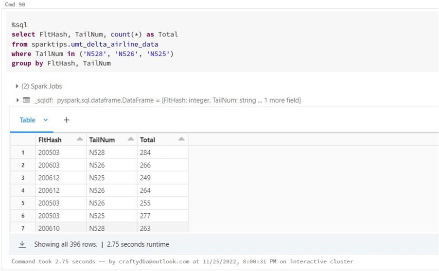
The last query below aggregates the number of flights for three planes over any given year and month. Thus, we are scanning all partitions, not just one. By the way, these three planes have the most logged trips in the database.
%sql
select FltHash, TailNum, count(*) as Total
from sparktips.mt_airline_data
where TailNum in ('N528', 'N526', 'N525')
group by FltHash, TailNum
The same output is generated for all queries (below). It only returns the 396 matching rows of data.
The table below shows the results of this testing effort.
| File Type | Run Time (sec) |
|---|---|
| AVRO | 15.42 |
| CSV | 23.98 |
| DELTA | 2.75 |
| JSON | 53.13 |
| ORC | 6.28 |
| PARQUET | 3.53 |
| TEMP VIEW | 35.67 |
I can only say that the temporary view has to infer the schema from the CSV files that are not partitioned. As a result, this format is in last place for two of the three tests. All other tests have Hive tables that supply the file schema, which increases performance. Both the delta and parquet formats perform well. They do not outshine the other formats when a single partition is selected for information gathering. It might be because there is always overhead of uncompressing the columnar format, and using a very small partition of the cluster for the query does not show any performance gain. On the other hand, when there are 256 partitions and each partition has to be searched, the delta and parquet formats are extremely fast.
Next Steps
The Spark engine supports seven different file formats. One format I did not talk about is the text format. I have used it in the past to parse log files. It is not used for structured data. Usually, regular expressions are used to find the needles in the haystack, better known as entries in the web server log file. Once a set of similar records is found, this data can be stored in another format.
Data file formats can be classified as either weak or strong. For example, the comma separated value format is considered weak because the schema has to be inferred by reading all the data, the information can be viewed with a text editor, the format can be broken by unwanted characters in a given row, and it does not natively support compression. The parquet file format is considered strong since it uses a strictly type binary format that supports columnar compression. Choosing the right file format is important for performance.
The Hive catalog supports two types of tables. The managed tables are stored where the Hive catalog is stored. Usually, this is stored in the default location (dbfs://user/hive). The unmanaged tables are predefined metadata for external files. A drop table on the managed type results in data loss. The same action on the unmanaged type results in the removal of metadata. Please remember that delta is the only format in which the Hive catalog is up to date with metadata and partitions. If you define a Hive table over existing partitioned data files, use the repair table option to update the catalog.
Performance testing is hard work. I could have spent much more time trying different options and/or queries. For instance, I did not restart the cluster for each query. Thus, I do not know if anything was already in cache. However, it is a known fact that Hive table definitions with predefined schema perform better than reads that must infer the data types. Also, Databricks has chosen the delta file format as a defacto for a data lake. Thus, the parquet format, which is a subset of delta, and the delta format should be your default file type. We saw that these file formats perform reasonably well.
Today, I started talking about Python functions. While I spend most of my day working in Spark SQL, I need to manipulate files. Thus, functions play an important role in creating reusable code. In fact, notebooks with correctly defined widgets (parameters) can be considered modules. In the future, I will show how some advanced problems can be easily solved using SQL functions built upon native Python libraries. Finally, enclosed is the notebook that contains the complete code used in this article.

John Miner is a Senior Data Architect at Insight Digital Innovation helping corporations solve their business needs with various data platform solutions.
He has over thirty years of data processing experience, and his architecture expertise encompasses all phases of the software project life cycle, including design, development, implementation, and maintenance of systems.
His credentials include undergraduate and graduate degrees in Computer Science from the University of Rhode Island. Also, he has earned certificates from Microsoft for Database Administration (MCDBA), System Administration (MCSA), Data Management & Analytics (MCSE), Data Science (MPP), Databricks Certified, and Fabric Certified.
John has been recognized with the Microsoft MVP award nine times for his outstanding contributions to the Data Platform community.
When he is not busy talking to local user groups or writing blog entries on new technology, he spends time with his wife and daughter enjoying outdoor activities. Some of John’s hobbies include wood working projects, crafting a good beer and playing a game of chess.
- MSSQLTips Awards: Author of the Year – 2019, 2022, 2023 | Champion (100+tips) – 2023