Understanding Spark DAG and Lazy Evaluation for Enhanced Performance

By: Anoop Kulkarni   |   Updated: 2024-01-19   |   Comments   |   Related: > Apache Spark

Problem

Apache Spark has revolutionized large-scale data processing with its distributed computing capabilities and efficient execution strategies. Among its key features, the Directed Acyclic Graph (DAG) and lazy evaluation are crucial in optimizing performance and resource utilization. Despite the inherent benefits of DAG and lazy evaluation, Spark applications can still face performance bottlenecks due to inefficient data shuffling, unnecessary transformations, and suboptimal execution plans. The main challenge lies in effectively harnessing the power of DAG and lazy evaluation to achieve optimal performance for diverse Spark applications.

Solution

To optimize Spark applications effectively, it is crucial to understand the underlying principles of DAG and lazy evaluation and their impact on performance. By carefully analyzing the execution plan and identifying potential bottlenecks, developers can implement strategies to minimize data shuffling, avoid unnecessary transformations, and optimize the order of operations. Techniques such as caching intermediate results, utilizing appropriate data partitioning schemes, and employing efficient transformation methods can significantly improve performance. Additionally, leveraging DAG visualization tools can provide valuable insights into the execution pipeline, facilitating further optimization efforts. By mastering a deep understanding of DAG and lazy evaluation, developers can harness the full potential of Spark to achieve optimal performance and efficiency in large-scale data processing tasks.

Understanding the Directed Acyclic Graph (DAG)

Spark's Directed Acyclic Graph (DAG) is a crucial component of its architecture, which is essential in optimizing performance and resource utilization during large-scale data processing tasks. To fully understand the significance of DAG, it's necessary to dive into its fundamental concepts and know how it influences Spark's execution strategy.

See the diagram below:

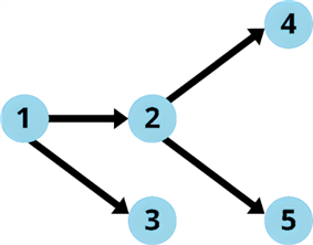
DAG is a visual representation of a sequence of tasks. It employs a graph structure, where circles represent individual tasks, and lines depict the flow of data or dependencies between them. Each circle is called a "vertex," and each line is an "edge." The term "directed" indicates that each edge has a defined direction, implying a one-way flow from one vertex to another. "Acyclic" signifies the absence of loops or cycles within the graph, ensuring that starting from any vertex and following the edges, you cannot return to the starting point. The entire structure of a DAG is visually represented as a graph.

In the context of Spark, it is a graph where nodes represent operations and directed edges represent the flow of data between them. The nodes represent Resilient Distributed Datasets (RDD), the basic data abstraction in Spark, while edges represent transformations applied to these RDDs.

For us to fully understand DAG and its functionality, we first need to understand a few concepts that are associated with it, such as RDDs, Transformations (Narrow and Wide), DAGScheduler and TaskScheduler, etc. that will be covered in later sections.

Resilient Distributed Dataset (RDD)

In Apache Spark, RDD and DAG are closely related concepts important in achieving efficient distributed data processing. RDDs represent the core data abstraction in Spark, while the DAG serves as a blueprint for executing operations on these RDDs. RDDs can be visualized as distinct points in a data processing pipeline, representing intermediate stages of transformation, aggregation, or filtering. Each RDD encapsulates a specific subset of the data, reflecting the operations applied to it.

RDDs are immutable, meaning that once an RDD is created, its data cannot be changed directly. Applying a new operation to an existing RDD creates a new RDD. This immutability is a crucial property of RDDs, contributing to fault tolerance and distributed processing capabilities. This immutability nature ensures that the data in an RDD remains consistent and predictable across all partitions and worker nodes in the Spark cluster. It eliminates the need for synchronization mechanisms, simplifying the parallelization and distribution of tasks.

The immutability of RDDs provides several benefits in the context of distributed data processing:

• Fault Tolerance: Immutability allows Spark to recover from failures efficiently by recreating lost partitions based on the lineage of operations. The unchanged state of RDDs ensures that the data remains consistent throughout the recovery process.
• Predictable Results: Since RDDs are immutable, the results of transformations are always predictable and deterministic. This predictability simplifies debugging and ensures that data is not unexpectedly modified during processing.
• Efficient Caching: Immutability allows Spark to cache RDDs effectively. Cached RDDs can be reused for subsequent transformations, improving performance by avoiding redundant computations.

Let's understand this with an example. See the code snippet below.

# Import libraries
from pyspark.sql.functions import avg
import pyspark.sql.functions as F
 
# Action: Reading a file is an action
df_data = spark.read.format("csv")\
        .option("header","true")\
        .load('/FileStore/employee.csv')
# Narrow transformation: Filter the dataset based on the Occupation
filtered_df = df_data.filter("Occupation='Teacher'")
 
# Narrow transformation: Filter the dataset based on the Age
filtered_age_df = filtered_df.filter(F.col("Age") >= 25).filter(F.col("Age") <= 30)
 
# Wide transformation: Calculate the average salary for each Gender
department_salary_df = filtered_age_df.groupBy("Gender").agg(avg("Salary"))
 
# Action: Show collects the data and outputs the result
department_salary_df.show()

This code snippet involves the following steps:

1. Reading a file: This action creates an RDD from the /FileStore/employee.csv file. Each partition of the RDD represents a portion of the data from the file.
2. Filtering the dataset: This narrow transformation filters the RDD based on the Occupation='Teacher' condition. It creates a new RDD containing only the rows where the Occupation column is equal to Teacher.
3. Further filtering: This is another narrow transformation that filters the RDD based on the age criteria (F.col("Age") >= 25) and (F.col("Age") <= 30). It creates a new RDD containing only the rows where the Age column is between 25 and 30, inclusive.
4. Grouping and aggregating: This is a wide transformation that groups the filtered RDD by the Gender column and calculates the average salary for each group using the agg(avg("Salary")) function. It creates a new RDD containing the average salary for each gender.
5. Showing the results: This action shows the final RDD (the one containing the average salary for each gender) and outputs the results.

Note: We will reference this code snippet in several subsequent sections.

Transformation and Actions

Each node in the DAG represents either a Transformation or an Action, each serving a distinct role in the data processing pipeline. Simply put, transformations modify the RDD, while actions trigger computations and return results.

Transformations

Transformations represent operations that modify or manipulate RDDs, the fundamental data abstraction in Spark. They are lazy operations - they are not executed immediately when applied to an RDD. Instead, they create new RDDs based on the input RDDs, but the actual computation is deferred until an action is triggered.

Examples of transformations include:

• map(): Applies a function to each element of an RDD.
• filter(): Filters out elements from an RDD based on a predicate.
• join(): Joins two RDDs based on a common key.

Furthermore, transformations can be categorized into two types: narrow and wide.

Narrow Transformations. Narrow transformations are transformations that do not shuffle the data – there is no movement of data between the partitions, and all operations happen on the same partition. This means that they can be executed without exchanging data between partitions. Narrow transformations are typically very efficient, as they do not require any additional overhead. Examples of narrow transformations include:

• map()
• filter()
• sample()

In the earlier-provided code snippet, the filtered_df = df_data.filter("Occupation='Teacher'") line is a narrow transformation. It filters the df_data DataFrame to only include rows where the Occupation column is equal to 'Teacher'. The resulting DataFrame, filtered_df, will have the same number of partitions as df_data.

Wide Transformations. Wide transformations shuffle the data, or that data is reorganized into new partitions. This means they change the data partitioning and may require exchanging data between partitions. Wide transformations can be more expensive than narrow transformations, as they can involve significant data movement. Examples of wide transformations include:

• reduceByKey()
• join()
• distinct()

In the code snippet provided, the department_salary_df = filtered_df.groupBy("Gender").agg(avg("Salary")) line is a wide transformation. It groups the filtered_df DataFrame by the Gender column and then calculates the average salary for each gender. The resulting DataFrame, department_salary_df, will have one column for each gender and one column for the average salary. The partitioning of the department_salary_df DataFrame may differ from the partitioning of the filtered_df DataFrame.

Actions

Conversely, actions trigger the actual computation of the RDDs and return a value to the driver program. They are terminating operations that bring the laziness of transformations to an end. Once an action is invoked, Spark constructs the DAG and executes the transformations in a pipelined fashion to achieve efficient data processing.

Examples of actions include:

• collect()
• show()
• read()

In the code snippet above, the show() action triggers the execution of the DAG and returns the filtered DataFrame as a result.

In Spark, transformations are lazy operations, meaning they do not perform any actual computation until an action is triggered. This allows Spark to build up a logical execution plan, or DAG, of the transformations that have been applied. So, the logical plan is constructed as the application code is parsed and interpreted before any actual computations are performed. When an action is triggered, Spark analyzes the DAG and determines the most efficient way to execute the transformations. Until an Action is encountered, Spark does not act upon any Transformations in the application code, and this operation is nothing but the lazy evaluation.

For the provided example, three jobs would be created-- one for each of the 'read', 'groupby' and 'avg' functions, and 'show'. Even though the 'groupby' and 'avg' functions are transformations, an additional Job is created during this operation. In a later section, we will see why and learn how to tackle this. So, during this process, DAG only creates a logical plan, which will be used later by the DAGScheduler to create the actual optimized execution plan.

DAGScheduler

The DAGScheduler is the high-level scheduling layer that translates a Spark application's logical execution plan into a physical one. It constructs a DAG of stages, where each stage represents a set of tasks that can be executed independently. The DAGScheduler also determines the preferred locations for running each task, considering data locality and resource availability. Further, the DAGScheduler analyzes the DAG to identify opportunities for optimization, aiming to minimize data shuffling and maximize parallel processing.

It applies various optimization techniques, such as pipeline execution, task reordering, and pruning unnecessary operations, to generate an optimized execution plan. This optimized plan is then submitted to the task scheduler, which schedules the tasks across the available worker nodes in the Spark cluster.

TaskScheduler

The TaskScheduler is the low-level scheduling layer in Spark responsible for running the tasks defined by the DAGScheduler. It interacts with the cluster manager (e.g., Mesos, YARN, or Spark Standalone) to acquire resources, allocate tasks to workers, and monitor task progress. The TaskScheduler also handles task failures, retries, and stragglers.

The DAGScheduler and TaskScheduler work in tandem to ensure the smooth execution of Spark jobs. The DAGScheduler provides the TaskScheduler with a structured plan of tasks, while the TaskScheduler handles the nuts and bolts of task execution and resource management. This division of work allows for efficient and scalable execution of Spark jobs on large clusters.

So, in a nutshell, Spark creates the DAG, which is a logical execution plan, and it immediately submits it to the DAGScheduler when an action is encountered. The DAGScheduler applies various optimization techniques, considers many other factors, and creates an optimized physical plan. It splits the graph into multiple stages based on the transformations in the application. All narrow transformations are grouped together into a single stage. However, when it sees a wide transformation, the DAGScheduler creates multiple stages and submits them to the TaskScheduler. Finally, the TaskScheduler makes sure the tasks are executed and monitored.

In summary, the DAGScheduler focuses on high-level planning and optimization, while the TaskScheduler handles the low-level execution details. Together, they enable Spark to process large datasets in a distributed manner efficiently. Before we dive into the next section, remember that the execution hierarchy is: 1) a Job is created for each DAG, 2) the Job is divided into different stages, and 3) each stage has one or more tasks, as shown in the diagram below.

Spark UI

The Spark UI, or Spark Web UI, is a web-based interface that provides a comprehensive overview of Spark applications, tasks, and cluster resources. It is a valuable tool for monitoring and debugging Spark applications, as it allows you to track the progress of jobs, identify bottlenecks, and analyze performance metrics.

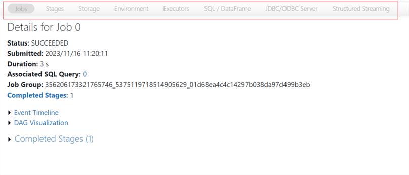
Key Features of the Spark UI

The Spark UI provides a wealth of information about the execution of Spark applications. Here are some of the key features:

• Jobs tab: A list of all the jobs submitted to the Spark cluster. You can see each job's name, status, start time, end time, duration, and some metrics.
• Stages tab: A list of all the stages executed by the Spark application. You can see each stage's name, status, input and output sizes, shuffle service information, and execution time.
• Tasks tab: A list of all the tasks executed by the Spark application. You can see each task's ID, status, start time, end time, duration, executor ID, machine ID, and metrics.
• Storage tab: Information about the storage used by the Spark application. You can see the total storage used and the storage used by each RDD and block.
• Environment tab: Information about the Spark application's environment. You can see the Spark version, the Scala version, the Java version, the Hadoop version, and the operating system.
• Executors tab: Information about the executors running the Spark application. You can see the ID of each executor, the machine ID, the memory used, the CPU used, and the tasks running on each executor.
• SQL tab: Information about the SQL queries executed by the Spark application. You can see the query text, the execution plan, and the metrics.

Furthermore, Spark UI can be used to monitor and debug Spark applications:

• Tracking the progress of jobs: Use the Jobs tab to track the progress of jobs and identify any jobs that are taking a long time to complete.
• Identifying bottlenecks: Use the Stages and Tasks tabs to identify bottlenecks in the execution of Spark applications.
• Analyzing performance metrics: Utilize the metrics displayed in the Spark UI to analyze the performance of Spark applications. For example, you can see how much CPU and memory each stage and task uses.
• Examining logs: Use the Spark UI to examine the logs for failed tasks and executors. This can help identify the cause of failures and debugging.

So far, we have covered all the theory needed to understand the DAG-Lazy evaluation. Now, let's jump to the practical part.

Job Execution Explained

Referencing the previous code snippet provided, we discussed that it creates three jobs. Next, we will explain each one, giving an in-depth understanding of how Spark executes jobs.

Job 0

The job is executed in a single stage, Stage 0.

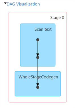
Stage 0 is responsible for reading the employee.csv file and creating a DataFrame. It consists of the following parts:

• Scan text: The job scans the text file and creates an RDD from the file.
• WholeStageCodegen: Spark uses a technique called whole-stage code generation (codegen) to generate efficient JAVA byte-code for each stage of a Spark job. Codegen can significantly improve the performance of Spark jobs, especially for jobs that involve complex transformations or large amounts of data.

In a nutshell, in Stage 0 of Job 0, Spark parsed the files and generated highly optimized Java bytecode.

Job 1

The job is executed in a single stage, Stage 1.

Stage 1 of the Spark job is responsible for reading the input data from the civ table, transforming the data, and writing the output data to a new dataframe. It consists of the following parts:

• Scan csv: Reads the CSV file into a Spark DataFrame.
• WholeStageCodegen: Generates optimized Java code for the job.
• Exchange: Shuffles the data across the cluster to be aggregated. This step exchanges data between executors. Spark executors are the distributed workers that execute Spark jobs. Spark jobs are divided into stages, and each stage is executed by a set of executors. In some cases, the data must be exchanged between executors to complete the stage. For example, if a stage performs a shuffle operation, the data must be exchanged between executors to group the data by key.

Job 2

The job is executed in a single stage, Stage 3, skipping Stage 2.

Stage 2 (Skipped). The Spark job in the image has two stages, but stage 2 is skipped. This is because the data required for Stage 3 is already available in memory from Stage 1.

Stage 1 scans a CSV file and reads it into memory as a Spark RDD. Stage 3 then performs an Adaptive Query Engine (AQE) shuffle read on the RDD from Stage 1. This shuffle read is necessary to redistribute the data across the executors to be processed in parallel.

However, since the data is already in memory from Stage 1, Spark does not need to re-execute Stage 2 to shuffle the data again. Instead, it can skip Stage 2 and use the data already in memory.

Stage 3. This stage scans the CSV file and reads it into Spark. The stage uses the WholeStageCodegen optimization to generate code for the entire stage at runtime. This can improve performance by reducing the overhead associated with interpreting code.

The job also uses the AQEShuffleRead operator to read the data from the CSV file. The AQEShuffleRead operator is a Spark optimization, which is part of AQE, a feature of Spark that allows the query optimizer to adjust the query plan at runtime based on the statistics of the data. This operator works by dividing the input data into small partitions and then shuffling those partitions across the cluster. This approach allows Spark to process the data in parallel, improving performance.

The AQEShuffleRead operator also uses a technique called "coalescing" to reduce the number of shuffle partitions. Coalescing combines multiple small partitions into a larger partition, which can reduce the overhead associated with shuffling data.

The most important thing to notice here is how Spark optimizes all these executions during the runtime.

Let's look at the diagram below.

As seen in the SQL tab, Spark intelligently combined multiple operations into a single statement. It has internally optimized the execution plan by combining both filter operations in our code into a single operation during runtime. All this is possible because of Spark's lazy evaluation.

Job Explanation

Now, you may ask why three jobs were created while only two actions ('read' and 'show') were in the code. Ideally, it should create only two jobs. It's a valid question; let's try to understand what happened.

There are a few reasons why Spark might create more jobs than the number of actions in your code. Here are a few possibilities:

1. Caching: If you cache any intermediate RDDs or DataFrames, Spark will create a separate job to materialize the cached data when needed.
2. Sampling: Spark uses sampling to estimate the size of RDDs and DataFrames. This can create a separate job, even if you don't explicitly call the sample() action.
3. Optimizations: Spark may sometimes create additional jobs to optimize the execution of the code. For example, it may create a separate job to perform shuffle operations.
4. Shuffle Operations: Spark may create separate jobs for shuffle operations, which involve exchanging data between partitions. If the code involves operations like groupBy or join, Spark might split the data into partitions and shuffle it across different executors to ensure efficient processing.

In our case, Spark created two jobs for the provided code because of how the groupBy() and agg() transformations are executed. When we call groupBy(), Spark creates a new RDD that contains the same data as the original RDD but with the records grouped by the specified column. However, this new RDD is not materialized until an action is triggered.

Here, the action is the agg() transformation, which calculates the average salary for each gender. When Spark executes the agg() transformation, it needs to materialize the grouped RDD, which involves performing a shuffle operation. This shuffle operation can be computationally expensive, so Spark breaks it down into multiple stages.

The first stage of the shuffle operation involves partitioning the data by gender. This is why we see the first job in the Spark UI. The second stage of the shuffle operation consists of aggregating the data within each partition. This is why we see the second job in the Spark UI.

To reduce the number of jobs in this case, we need to use the coalesce() transformation to reduce the number of partitions in the RDD to 1, reducing the amount of data to be shuffled, hence improving the performance of the Spark job.

Updated code snippet:

# Import libraries
from pyspark.sql.functions import avg
import pyspark.sql.functions as F
 
# Action: Reading a file is an action
df_data = spark.read.format("csv")\
        .option("header","true")\
        .load('/FileStore/employee.csv')
# Narrow transformation: Filter the dataset based on the Occupation
filtered_df = df_data.filter("Occupation='Teacher'")
 
# Narrow transformation: Filter the dataset based on the Age
filtered_age_df = filtered_df.filter(F.col("Age") >= 25).filter(F.col("Age") <= 30)
 
# Wide transformation: Calculate the average salary for each Gender
# department_salary_df = filtered_age_df.groupBy("Gender").agg(avg("Salary"))
 
# Coalesce to reduce the partition
department_salary_df = filtered_age_df.coalesce(1).groupBy("Gender").agg(avg("Salary"))
 
# Action: Show collects the data and outputs the result
department_salary_df.show()

However, Spark sometimes creates more jobs than the actions it has encountered in a code. The following are some steps one can take to debug why that is happening:

1. Inspect stages of your job: In the Spark UI, go to the Jobs tab to see a list of all the jobs in your application. For each job, you can see the number of stages and the duration of each stage.
2. Evaluate a stage: To see more details about a stage, click on the arrow next to the stage name to expand the stage and show you the tasks that are executed in the stage.
3. Verify task durations: The duration of a task is the amount of time it takes to execute the task. If a task is taking a long time, it may be causing Spark to create additional jobs.
4. Check task details: Click on the task name to see more details about a task, including input and output data for the task and the stack trace for the task.

Overall, the synergy between DAG and lazy evaluation empowers Spark to optimize performance in several ways:

• Minimizes Data Shuffling: DAG identifies the dependencies between tasks, enabling Spark to schedule them strategically to minimize data movement across the cluster.
• Eliminates Redundant Computations: Lazy evaluation ensures that computations are performed only when their results are required, preventing unnecessary work and reducing overhead.
• Caches Intermediate Results: Spark can cache intermediate results to avoid recomputing them repeatedly, further reducing processing time.

DAGs Fault Tolerance and Lineage

DAGs also play a crucial role in Spark's fault tolerance mechanisms. Spark can recover lost data or recompute failed tasks by tracking lineage information, which captures the dependencies between RDDs, without restarting the entire job. This feature ensures that Spark applications can continue running despite node failures or network interruptions.

RDD recovery is another important aspect of DAGs. When an RDD partition is lost due to a node failure, Spark can reconstruct it based on its lineage information. This process ensures that the application can proceed without losing data.

DAGs also facilitate lineage maintenance, which is crucial for maintaining the integrity of Spark applications. Lineage information allows Spark to track the origin of each RDD and identify the operations that produced it. This information is essential for debugging purposes and ensuring that Spark application results are consistent, even in the event of failures.

Conclusion

Apache Spark's DAG and lazy evaluation techniques provide a powerful foundation for optimizing performance and resource utilization in large-scale data processing. However, effectively harnessing these capabilities requires careful analysis and optimization strategies to address potential bottlenecks such as inefficient data shuffling, unnecessary transformations, and suboptimal execution plans. Developers can achieve optimal performance by leveraging DAG visualization tools, understanding the impact of data partitioning schemes, and implementing efficient transformation methods. Mastering the principles of DAG and lazy evaluation empowers developers to fully exploit Spark's capabilities for efficient and scalable data processing.

Next Steps

• Understanding your Apache Spark application through visualization
• Understand Spark's Web UI

About the author

Anoop Kulkarni is a Microsoft Certified Data Engineer with 13+ years of experience in Data Engineering.

This author pledges the content of this article is based on professional experience and not AI generated.

View all my tips