By: Harris Amjad | Updated: 2023-05-19 | Comments (2) | Related: > Power BI
Problem
Sometimes one needs multiple relations between the same tables in a Microsoft Power BI dashboard. However, in modeling, you will see that Power BI makes one of the relationships inactive during a calculation or visualization. This tutorial highlights the DAX function, which assists in making inactive relations active as per the need of the calculation or visualization. This tutorial will act as a step-by-step guide to using DAX to assist in creating multiple relations between the same table in Power BI desktop for business intelligence projects.
Solution
With the advent of the big data revolution, our world has become highly saturated with large volumes of information, which continues to evolve our data needs and related technologies. To ensure that different entities efficiently leverage this data, we use a computerized system of storing and extracting data through a database management system (DBMS). As an overview, databases consist of different tables in which each row can be uniquely identified by a specific column (field) known as the primary key. However, a relational database's real power and structure lies in establishing relationships between its tables. By connecting related data across tables, one can create complex and meaningful queries that allow you to extract valuable insights for data analysis. This tutorial will assess how to create multiple relationships between the same tables in Power BI.
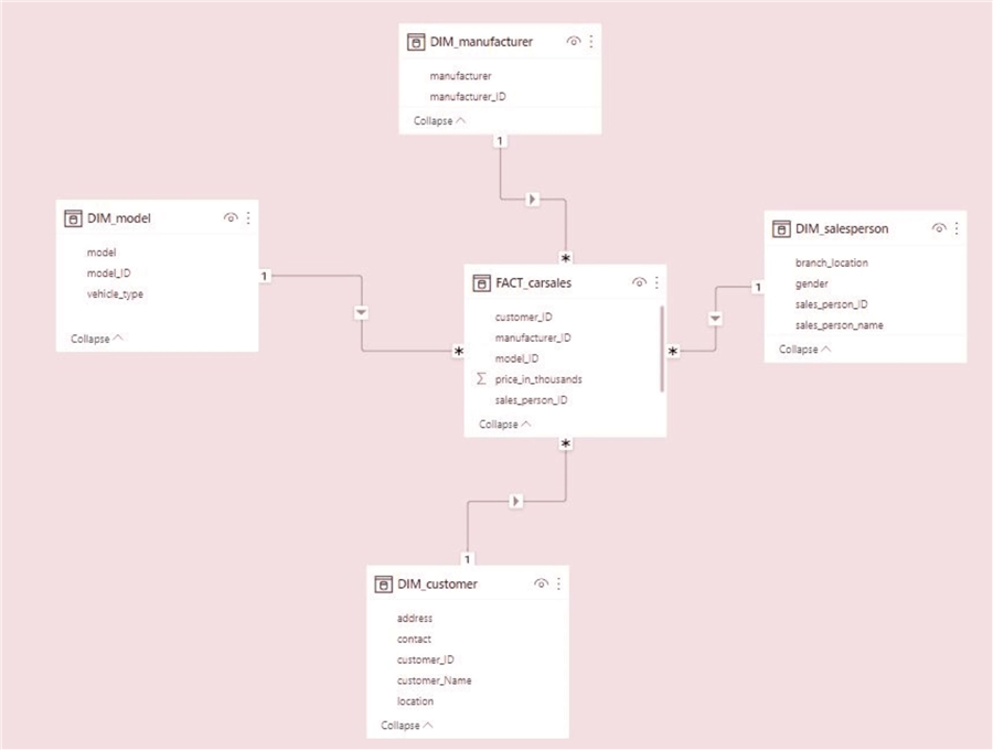
For example, in the above picture, we can see the Power BI data model, allowing us to observe how the data is organized and related to each other within a database. Each block represents a table alongside its relevant fields/columns. More importantly, the lines and arrows between the tables signify a cardinality relationship within the schema. It is also interesting to note that these lines are marked with a '1' and '*'. What does this mean?
These symbols refer to the different types of relationships in a database. They can be:
- One-to-One: This relationship exists when a single record in one table is related to only one record in another table and vice versa. For example, let's say you organize information about your employees and want to keep track of their passports. This is a classic example of a one-to-one relationship, as each person can only have a single passport, and each passport is issued to only one person. Such relationships, however, tend to be uncommon as we can easily store corresponding information in the same table. In the example above, a line connected by two '1's on either side will signify this type of relationship.
- One-to-Many: This relationship exists when a single record in one table can be related to multiple records in another table. However, each record in the second table can only be related to one record in the first table. An example of this relationship would be customers and their orders. A single customer can place multiple orders; however, each order only belongs to one customer. This is the most common type of database relationship, and in the schema above, it is represented by an '*' and a '1' between the relevant tables.
- Many-to-Many: This relationship exists when multiple records in one table can be related to multiple records in another table. For instance, in a publishing company's database, the authors and books may have a many-to-many relationship as each book can be written by several authors, and each author can also write several books. A junction table is utilized in normal use cases to prevent data duplication. It typically includes two foreign keys that reference the primary keys of the original tables, along with any additional fields specific to the relationship between the two tables. This relationship is signified by two '*' on either side of the line in the schema above.
Considering the wide diversity of DBMS use cases, it is possible that multiple relationships of the types we have discussed above may originate from our tables. We will now outline a practical demonstration whereby we will create a schema in MySQL and then observe and manipulate our data model in Power BI.
Creating a Schema in MySQL
For this demonstration, we are concerned with the monthly sales of a bookstore. Currently, our schema will be comprised of a single table with the following fields:
- Order date
- Shipping date
- Product key
- Customer ID
- Total sales made
To get started, we will first create our database and then access it using the following commands:
CREATE DATABASE bookstore_sales;
USE bookstore_sales;
Now, we will create our table using the following statements, which will include the fields mentioned above:
CREATE TABLE monthly_sales
(
    order_date date,
    ship_date date,
    product_key varchar(6),
    customer_id varchar(8),
    sales int unsigned
);
Now that we have a skeletal structure for our table, we can populate it by executing the following commands:
INSERT INTO monthly_sales VALUES
("2023-02-01", "2023-02-02", "BK1234", "LHR78902", 20),
("2023-02-02", "2023-02-02", "BK4568", "LHR34901", 50),
("2023-02-04", "2023-02-04", "MV1890", "KHI17392", 30),
("2023-02-04", "2023-02-05", "BK0098", "LHR19028", 10),
("2023-02-05", "2023-02-05", "MV2900", "RWP16370", 60),
("2023-02-06", "2023-02-07", "MG1902", "MUL29104", 30),
("2023-02-09", "2023-02-15", "MG1839", "SIA38291", 40),
("2023-02-10", "2023-02-15", "BK2891", "LHR00382", 80),
("2023-02-14", "2023-02-15", "BK0032", "ISL10394", 30),
("2023-02-15", "2023-02-15", "MV9001", "LHR01919", 20),
("2023-02-18", "2023-02-20", "MV8834", "MUL18301", 50),
("2023-02-20", "2023-02-20", "MG0219", "KHI32413", 40),
("2023-02-22", "2023-02-27", "BK6002", "ISL90029", 80),
("2023-02-23", "2023-02-27", "BK9921", "BWP82716", 60),
("2023-02-26", "2023-02-27", "MG0192", "LHR10284", 40);
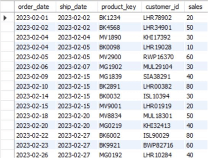
Lastly, we can inspect our table using the SELECT statement in MySQL:
SELECT * FROM bookstore_sales.monthly_sales;
This will output our source table, as seen below.
Multiple Relationships in Power BI
Now that we have a database, we can import it into Power BI to observe multiple relationships emerging between the same tables.
Step 1
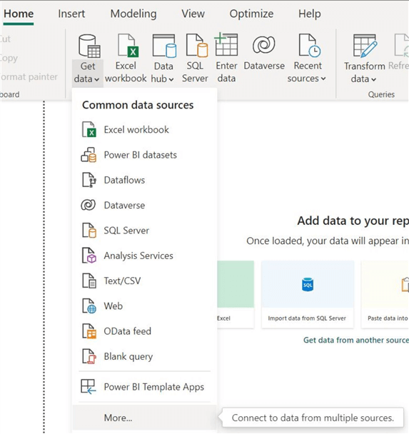
Before we can delve into the essence of our topic, we need to import our database from MySQL to Power BI. To do that, click Get data in the Home ribbon and click More… at the bottom of the resulting list. As shown below, we can observe a range of common data sources we can work with in Power BI.
Step 2
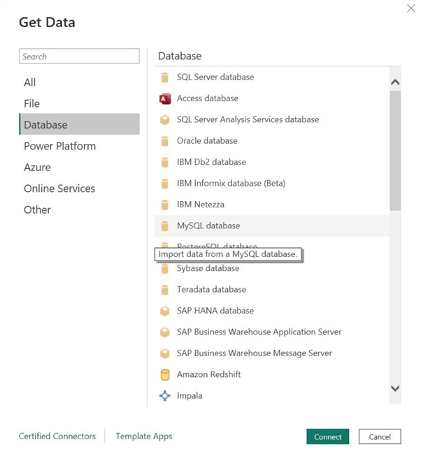
The Get Data window will appear. Below the search box, select the Database category and choose the MySQL database option towards the right, as shown below. Then click Connect at the bottom of the window. This step is flexible depending on the platform your database is hosted on.
Step 3
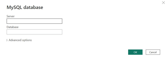
The MySQL database window will appear. Enter the relevant server and database credentials in the dialog boxes and click OK.
Step 4
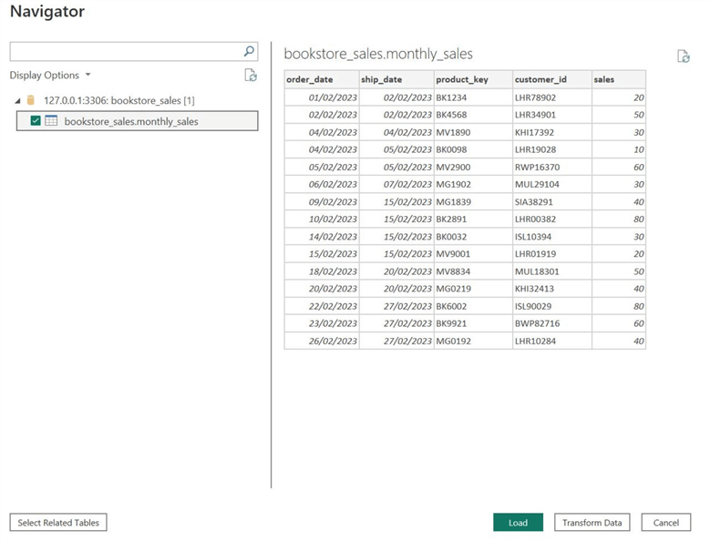
The Navigator window will pop up if Power BI successfully connects with your database. Below Display Options, check the selection box beside the "bookstore_sales.monthly_sales" table and click Load at the bottom of the window. Power BI also enables users to observe the tables they are loading, as shown below. If there are any anomalies with the dataset, we can also cater to that using the Transform Data option at the bottom of the window, which will take us to a Power Query Editor window, where tools are available to manipulate our dataset. However, we don't need to delve into that as our database is complete and clean.
Step 5
After successfully loading our selected tables to Power BI, we are ready to move toward the essence of our main problem. Currently, our database only consists of a single table. As it is a single entity, there is no possibility for database relationships.
For our purposes, we will focus on book sales by shipping and orders. Before we can compute these numbers, we must create a date table that encodes all information regarding the dates required in this dataset. It will include a date column encompassing year, quarter, month, and day alongside separate columns for "month", "year", "month index", and a "yearmonth" field that captures concatenated year and month.
In the main interface of Power BI, under the Modeling ribbon, click New table, as shown below.

In the formula box, enter the following DAX formula and click Enter:
DateTable =
   GENERATE (
      CALENDAR ( DATE ( 2023, 2, 1 ), DATE ( 2023, 2, 28 ) ),
      VAR currentDay = [Date]
      VAR startYear = 2023
      VAR month =  MONTH ( currentDay )
      VAR year =  YEAR ( currentDay )
   RETURN   ROW (
      "month", month,
      "year", year,
      "month index", INT ( ( year - startYear ) * 12 + month ),
      "YearMonth", year * 100 + month  )
 )
Step 6
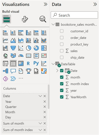
Select the Table icon in the Visualizations panel to observe our newly created table, as shown below. This is a pre-built visual, and we can populate it by selecting or dragging all the columns of the "DateTable" to the "Columns" field, as shown below.
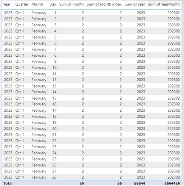
We can now see our table in the main working space of Power BI, presented below.
Step 7
Now that we have two tables in our database, there is a possibility of relationships between them. Click the Model view icon towards the right (see below) to visualize our current database schema.
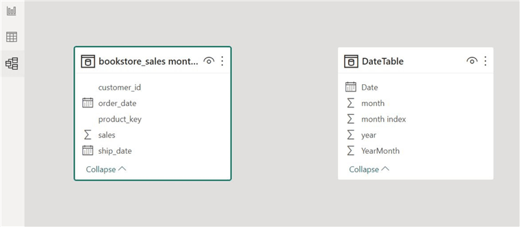
To establish relationships between the same tables, drag the "Date" column from our "DateTable" and connect it to the "order_date" column of the other table. This will create our first relationship. For our second one, again drag the "Date" column and connect it to the "ship_date" column of our "monthly_sales" table. This process is outlined below:
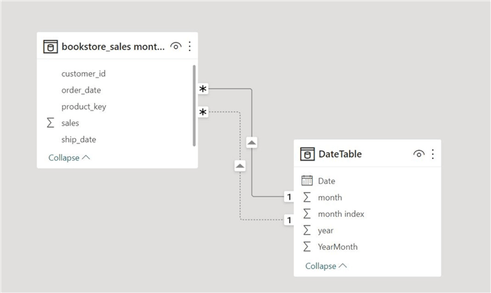
We can observe that the "DateTable" and "monthly_sales" tables have two one-to-many relationships. However, it is interesting to note that the relationship between the "Date" and "ship_date" is rendered inactive (shown by the dashed line) as Power BI only allows one active connection between the tables.
Step 8
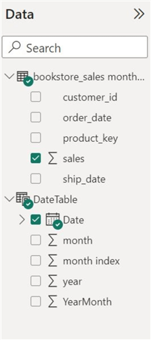
We now need to figure out a method to utilize the inactive relationship. To see what our data is doing, we can go back to our report view panel, where on another page, we will be creating a new table visual. After selecting the Table icon, we can once again populate our "columns" field by selecting the "Date" and "Sales" columns as outlined below.
Our resulting table is as follows:
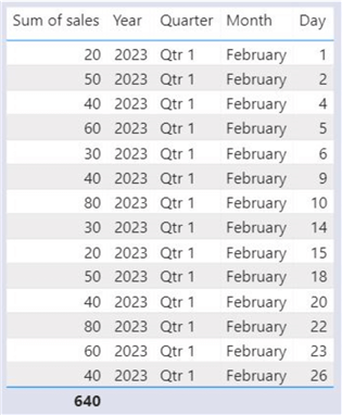
We can see how the data is categorized and how the sales add up to 640 units. What if we want to distinguish the sales by order date and shipping date?
Step 9
We need to compute two separate measures that sum up the sales by order dates and shipping dates. To do so, in the Home ribbon, click on New measure, as shown below:

To create our first measure that explicitly sums sales by order dates, enter the following DAX formula in the formula bar:
OrderDateSales =
   CALCULATE (
   SUM ('bookstore_sales monthly_sales'[Sales] ),
   USERELATIONSHIP ( 'DateTable'[Date], 'bookstore_sales monthly_sales'[order_date] )
   )
To create the other measure for sales by shipping dates, repeat the above process with the following DAX formula:
ShipDateSales =
   CALCULATE (
   SUM ('bookstore_sales monthly_sales'[Sales] ),
   USERELATIONSHIP ( 'DateTable'[Date], 'bookstore_sales monthly_sales'[ship_date] )
   )
Step 10
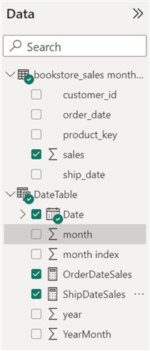
Now that we have our explicitly calculated measures, create another table visual and populate it with the "sales" and "Date" columns like before, but for the new measures as shown below.
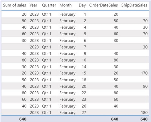
We can now see (below) that our book sales have been categorized according to the order dates and shipping dates, and all of them add up to our initial total of 640 units. This offers clarity that our calculation is working properly.
Step 11
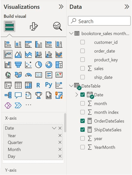
We can also visualize the two relationships using different graphical visuals like a line chart. Select the Line chart icon in the Visualizations panel and populate the "X-axis" field with the "Date" column, as shown below. For the "Y-axis," select the "OrderDateSales" and "ShipDateSales" measures.
After a few customizations, below is our new visual:
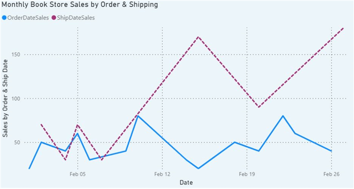
We can now clearly observe that for most of February, the bookstore shipped a larger volume of sales than it took orders. In other words, the store consistently took orders throughout the month but preferred to ship in bulk, reducing shipping costs and increasing efficiency, thus optimizing their supply chain strategy.
Conclusion
In this tip, we have discussed some of the fundamentals of databases, including the different types of database relationships. We then extended this concept to the possibility of multiple relationships between the same tables. We practically demonstrated that by building a schema in MySQL and manipulating it in Microsoft's Power BI.
Next Steps
- Check out all the Power BI Tips on MSSQLTips.com
Learn more about Power BI in this 3 hour training course.
About the author
 Harris Amjad is a BI Artist, developing complete data-driven operating systems from ETL to Data Visualization.
This author pledges the content of this article is based on professional experience and not AI generated.
View all my tips
Article Last Updated: 2023-05-19


