Problem
Partitioning data in Microsoft Fabric can significantly optimize performance for large datasets by enabling faster query execution, streamlined data management, and reduced storage costs. In this article, we’ll explore some ways to implement partitioning within Microsoft Fabric, illustrating with examples in Lakehouses, Warehouses, and Pipelines.
Although Dataflows Gen2 in Microsoft Fabric can also support data partitioning, the approach is more focused on filtering and exporting data into partitioned storage rather than directly defining partitions like in traditional databases.
Solution
Partitioning divides data into smaller, manageable segments, organizing it logically and physically. Instead of processing entire datasets, queries focus only on relevant partitions. This approach provides:
- Improved Query Speed: Scans only the relevant data, reducing latency.
- Cost Savings: Decreases computational overhead by narrowing the query scope.
- Streamlined Management: Simplifies operations, like incremental loading, archiving, and data governance.
In Microsoft Fabric, partitioning can be implemented across:
- Lakehouses: Partitioning file-based data (e.g., Parquet) stored in lake storage.
- SQL Warehouses: Partitioning relational tables for optimized query processing. There are some limitations to implementing this in a Fabric Warehouse compared to Azure Synapse at the time of writing. This and a workaround will be discussed more in this article.
- Pipelines: Dynamic partitioning during ingestion or data transformation.
Let’s examine each method with actionable steps and examples using the Customers-100000 csv dataset.
Prerequisites
The following assumptions have been made for better understanding and to easily follow along:
- A Fabric Workspace has been created.
- A Fabric Lakehouse has been created.
- A Fabric Warehouse has been created.
- You have a Fabric license or a Fabric Trial.
See this article about how to set up a Lakehouse architecture in Microsoft Fabric.
Partitioning in a Lakehouse (Data Lake)
Let’s say we have a large dataset in the Customers-100000 csv, and we want to partition it by Year, Month, and Day in a Fabric Lakehouse. Assuming the dataset is initially uploaded into a Lakehouse ‘File‘ called ‘raw_data’. Check out this tip on how to upload your downloaded datasets to a Fabric ‘File’ subfolder.
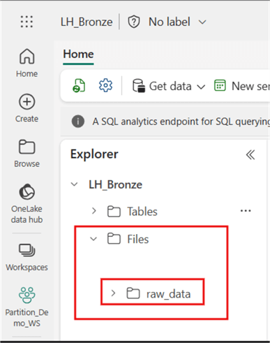
The image below shows my ‘raw_data’ subfolder in a Lakehouse named ‘LH_Bronze’. The assumption is that the raw customer data would be periodically uploaded into the ‘raw_data’ subfolder as it is.
Steps for Partitioning Data in Lakehouse
You might prefer to partition the data within the Lakehouse ‘Files’ in the Bronze Layer, a popular choice; however, this is based on your architectural plans and requirements. The following steps describe how to achieve partitioning in a Lakehouse File.
- Prepare Data: Use Spark or any other compute engine in Microsoft Fabric to load the data and structure it according to the required partitioning columns.
- Define Partition Columns: Specify the Year, Month, and Day columns in the data.
- Write Data to Lakehouse File Location: When writing data to the Lakehouse, specify the partitioning structure so that Fabric can physically store the data in separate folders.
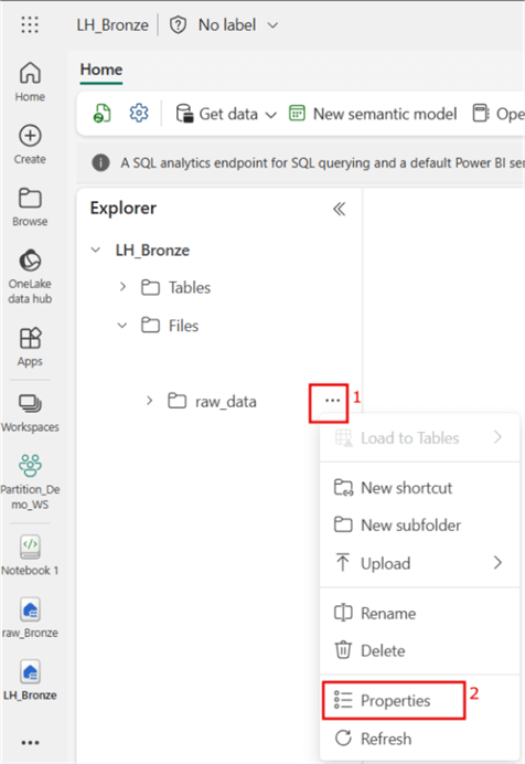
The three steps above have been encoded in the Spark code below. Note that a ‘Notebook’ is needed in the Lakehouse to write the code. (Please refer to the earlier mentioned article as a guide.) To get the ABFS (Azure Blob Filesystem) source path, navigate to the Lakehouse File, click the ellipses (…) at the end of ‘raw_data’, and click Properties, as seen in the image below.
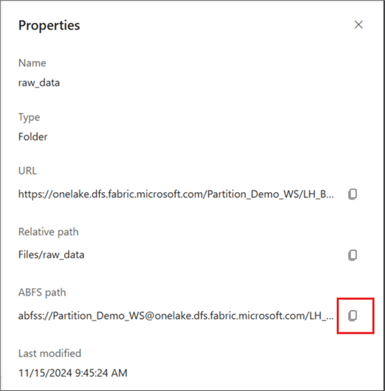
In the Properties window, copy the ABFS path, as seen in the image below. You will need this path at the “Define ABFS Path for source files in Lakehouse” line of code.
#### Script to partition dataset into Lakehouse files ####

from pyspark.sql import SparkSession
from pyspark.sql.functions import col, to_timestamp, date_format
from notebookutils import mssparkutils

# Initialize SparkSession
spark = SparkSession.builder.getOrCreate()

# Define ABFS Path for source files in Lakehouse
abfs_path = "abfss://Partition_Demo_WS@onelake.dfs.fabric.microsoft.com/LH_Bronze.Lakehouse/Files/raw_data"

# Load data from Lakehouse folder into a DataFrame
df = spark.read.format("csv").option("header", "true").load(abfs_path)

# Verify schema and data quality - this is optional but might help if you need to read this data into a Data Warehouse table later.
df.printSchema()  # Optional: Display the schema
df.show(5)        # Optional: Preview data to verify the structure

# Define output folder in Lakehouse (for readability)
output_folder = 'output_partitioning'

# Define ABFS output path for the partitioned files
output_path = f"abfss://Partition_Demo_WS@onelake.dfs.fabric.microsoft.com/LH_Bronze.Lakehouse/Files/{output_folder}"

# Add new columns to the DataFrame (year, month, and day)
df_output = (
    df.withColumn("Subscription Date", to_timestamp(col("Subscription Date")))  # Convert to timestamp
      .withColumn("day", date_format(col("Subscription Date"), "dd"))   # Extract day
      .withColumn("year", date_format(col("Subscription Date"), "yyyy"))  # Extract year
      .withColumn("month", date_format(col("Subscription Date"), "MM"))   # Extract month
)

# Verify the transformed data
df_output.select('day', 'month', 'year').show(5)  # Show a sample of the partition columns

# Write data into Lakehouse with partitioning by 'year', 'month' and 'day'
df_output.write.mode("append").partitionBy('year','month','day').parquet(output_path)

# Confirm successful write operation (optional)
print(f"Data successfully written to {output_path}")
So, as you can see in the PySpark code above, I have planned to write the partitioned files into a Lakehouse File subfolder known as ‘output_partitioning‘ as seen by the line of code below (which is part of the block of code above).
# Define output folder in Lakehouse (for readability)
output_folder = 'output_partitioning'

# Define ABFS output path for the partitioned files
output_path = f"abfss://Partition_Demo_WS@onelake.dfs.fabric.microsoft.com/LH_Bronze.Lakehouse/Files/{output_folder}"
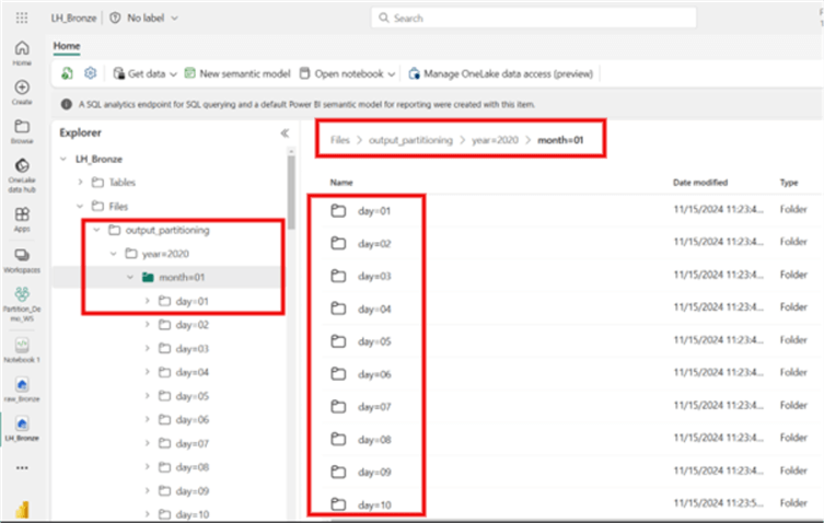
Once the PySpark code runs, the output creates the ‘output_partitioning’ subfolder and then partitions the data by Year, Month, and Day, as seen in the image below.
What are the Benefits of Partitioning on Lakehouse Files
- Queries filtering by Year and Month will only scan relevant folders, improving read performance.
- Data is logically organized, making it easier to manage and optimize.
Partitioning in a Microsoft Fabric SQL Warehouse
Partitioning in a SQL Warehouse allows for efficient querying of relational tables. However, as mentioned earlier, Microsoft Fabric’s Warehouse currently does not natively support partitioning tables using RANGE or HASH partitioning like other relational databases. However, alternative approaches can be adopted to achieve similar benefits for managing large datasets effectively.
One alternative approach I found to be efficient is when working with Lakehouse alongside SQL Warehouse in Fabric. You can offload partitioning responsibilities to the Lakehouse and query the data using Direct Lake mode. The steps to achieve this are as follows.
Step 1: Partition the Data into a Lakehouse Table
Partition data by writing it to the Lakehouse table using Spark, as shown in the PySpark code below.
#### Script to partition dataset into Lakehouse table ####

from pyspark.sql import SparkSession
from pyspark.sql.functions import col, to_timestamp, date_format

# Initialize SparkSession
spark = SparkSession.builder.getOrCreate()

# Define ABFS Path for source files in Lakehouse
abfs_path = "abfss://Partition_Demo_WS@onelake.dfs.fabric.microsoft.com/LH_Bronze.Lakehouse/Files/raw_data"

# Load data from Lakehouse folder into a DataFrame
df = spark.read.format("csv").option("header", "true").load(abfs_path)

# Print the schema and preview the data (optional)
df.printSchema()
df.show(5)

# Transform the data
# Ensure column naming and timestamp transformation
df_output = (
    df.withColumn("Subscription_Date", to_timestamp(col("Subscription Date")))  # Convert to timestamp
      .drop("Subscription Date")                                               # Remove the original column
      .withColumn("day", date_format(col("Subscription_Date"), "dd"))          # Extract day
      .withColumn("year", date_format(col("Subscription_Date"), "yyyy"))       # Extract year
      .withColumn("month", date_format(col("Subscription_Date"), "MM"))        # Extract month
)

# Rename columns to replace invalid characters
df_output = df_output.select(
    *[col(c).alias(c.replace(" ", "_").replace(",", "").replace("(", "").replace(")", "")) for c in df_output.columns]
)

# Verify the transformed and renamed data
df_output.printSchema()
df_output.show(5)

# Define ABFS path for Delta table
delta_table_path = "abfss://Partition_Demo_WS@onelake.dfs.fabric.microsoft.com/LH_Bronze.Lakehouse/Tables/Partitioned_Delta_Table"

# Write the data into a Delta table, partitioned by 'year', 'month', and 'day'
df_output.write     .mode("overwrite")     .partitionBy('year', 'month', 'day')     .format("delta")     .save(delta_table_path)

# (Optional) Register the Delta table in the metastore
spark.sql(f"CREATE TABLE IF NOT EXISTS Partitioned_Delta_Table USING DELTA LOCATION '{delta_table_path}'")

print("Data successfully written to Delta Lake table!")
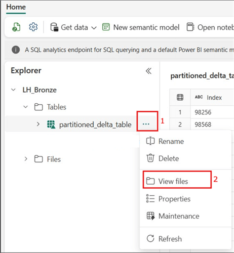
The image below shows the partitioned table in a Lakehouse table, including the partitions up to the ‘day’ granularity. Note: To expose the partitions, click on the ellipses (…) at the end of the created table and select View files.
Step 2: Expose Lakehouse Table Data in the Warehouse
First, create a table schema in the Warehouse. For this demonstration, a table named Partition_Table has been created, as seen in the code below.
CREATE TABLE Partition_Table
(
    Index_Num INT,
    Customer_Id VARCHAR(255),
    First_Name VARCHAR(255),
    Last_Name VARCHAR(255),
    Company VARCHAR(255),
    City VARCHAR(255),
    Country VARCHAR(255),
    Phone_1 VARCHAR(255),
    Phone_2 VARCHAR(255),
    Email VARCHAR(255),
    Subscription_Date DATE,
    Website VARCHAR(255),
    day INT,
    month INT,
    year INT
);
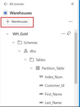
To link the Warehouse to the Lakehouse where the partitioned table was created, perform the following steps in the image below.
Click Warehouses.
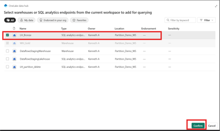
Select the Lakehouse where the partitioned delta table is created; in this case, it’s the ‘LH_Bronze’ Lakehouse, as seen in the image below. Click Confirm.
Step 3: Load and Query the Partitioned Data in the Warehouse
Since the data is partitioned in the Lakehouse, queries with filters (e.g., by Year) will benefit from partition pruning. But before that, we need to create a Stored Procedure to load partitioned data from the Lakehouse to the Warehouse.
The SQL Stored Procedure below helps to load the Warehouse table with the partitioned data in the Lakehouse.
CREATE PROCEDURE usp_Partitioned
AS
-- Step 1: Get the current maximum Index_Num
DECLARE @max_index INT;
SELECT @max_index = ISNULL(MAX(Index_Num), 0) FROM Partition_Table;

-- Step 2: Insert new data with incrementing Index_Num
INSERT INTO Partition_Table (Index_Num, Customer_Id, First_Name, Last_Name, Company, City, Country, Phone_1, Phone_2, Email, Subscription_Date, Website, day, month, year)
SELECT
    ROW_NUMBER() OVER (ORDER BY Customer_Id) + @max_index AS Index_Num,  -- Start incrementing from the max value
    Customer_Id,
    First_Name,
    Last_Name,
    Company,
    City,
    Country,
    Phone_1,
    Phone_2,
    Email,
    Subscription_Date,
    Website,
    day,
    month,
    year
FROM LH_Bronze.dbo.Partitioned_Delta_Table as silver
WHERE NOT EXISTS(
    SELECT 1
    FROM Partition_Table as pt
    WHERE pt.Customer_Id = silver.Customer_Id
);
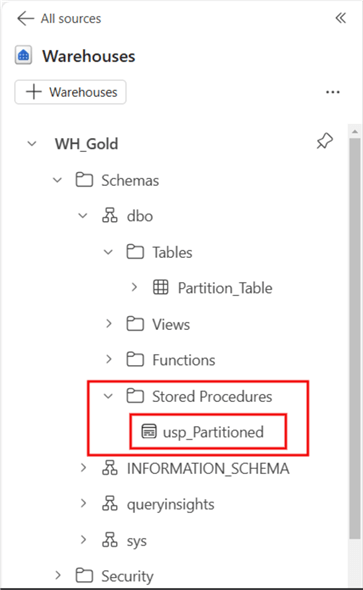
The image below shows where to find the Stored Procedure in the Warehouse.
Next, execute the Stored Procedure:
EXECUTE usp_PartitionedThen run a simple SQL script, like the one below, to return only the 2021 partition.
SELECT [Index_Num],
            [Customer_Id],
            [First_Name],
            [Last_Name],
            [Company],
            [City],
            [Country],
            [Phone_1],
            [Phone_2],
            [Email],
            [Subscription_Date],
            [Website],
            [day],
            [month],
            [year]
FROM [WH_Gold].[dbo].[Partition_Table]
WHERE year = 2021
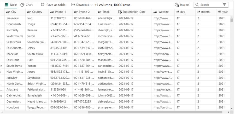
The output of the SQL script above should look like the image below.
Partitioning in a Microsoft Fabric Pipelines
When ingesting data via Pipelines in Microsoft Fabric, you can dynamically create partitions in the Copy Activity based on date or other criteria. This is particularly useful when loading data to a Lakehouse or a SQL Warehouse.
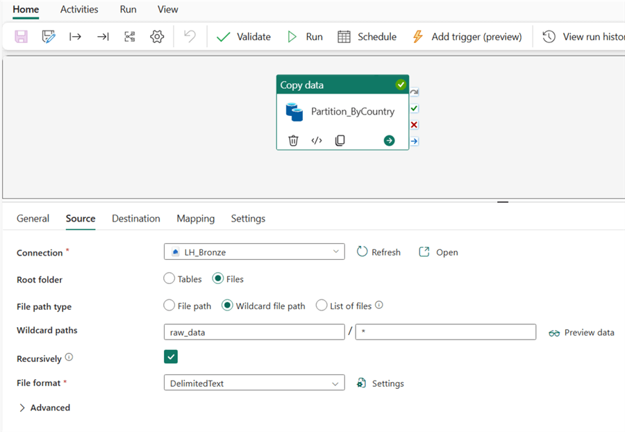
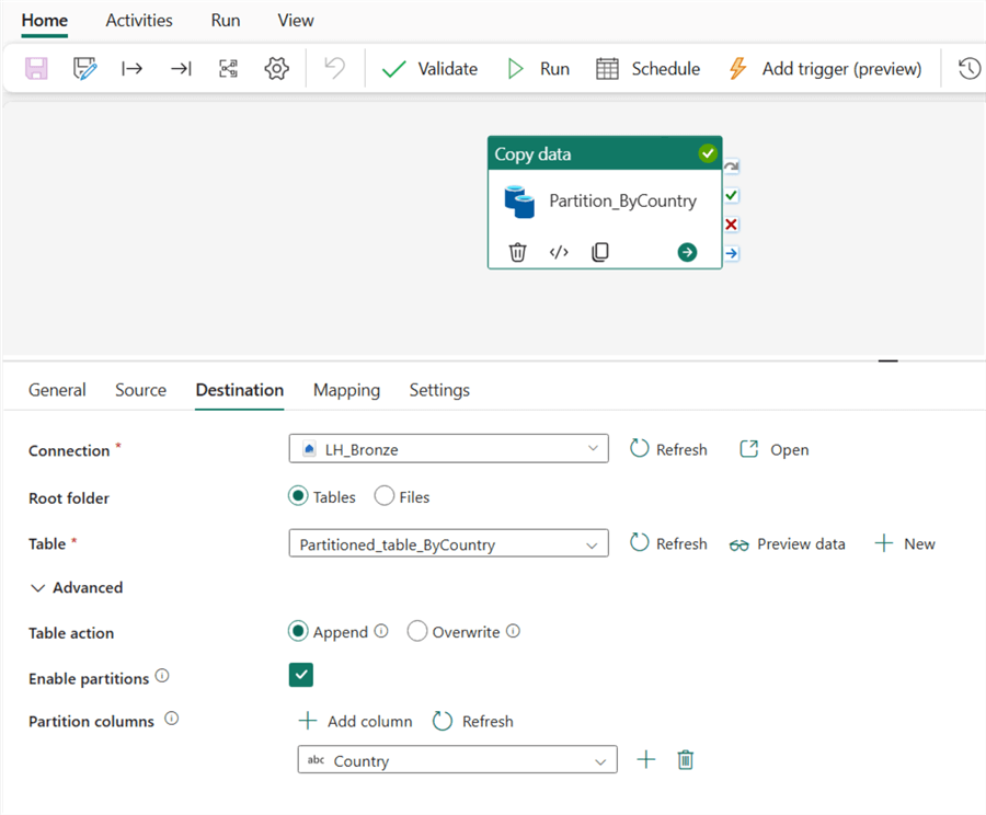
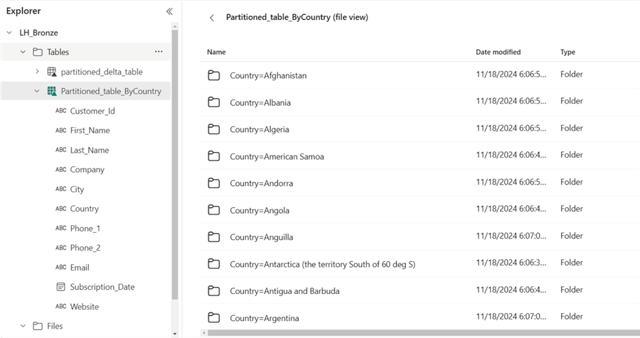
For this example, the Copy Activity in Fabric Pipelines will be used to partition this dataset by ‘Country‘.
For details concerning how to set up and configure a Copy Activity, please refer to the Microsoft Documentation.
The image below shows how this example is connected to the source in the Copy Activity.
The next image shows how the sink or Destination was configured in the Copy Activity.
Below shows how the mapping settings were configured.
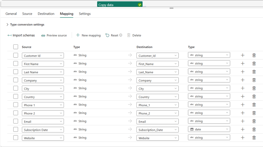
Afterward, the pipeline was validated and ran. The image below shows the partitioned data by country.
Considerations
Choice of Partition Key
Selecting an appropriate column for partitioning is critical. Avoid low-selectivity columns like Country or Gender, as they can lead to data skew, with some partitions being disproportionately large. Instead, prioritize high-cardinality columns such as Date, Region, or Department, which distribute data more evenly and reduce query processing times.
Dynamic Partitioning
Use dynamic strategies, such as partitioning by Year, Month, and Day, to handle time-series data efficiently. This approach is especially useful for incremental data loading and time-based querying, as it helps manage data growth while maintaining performance.
Uniform Data Distribution
Ensure balanced partition sizes to maximize query performance. Skewed partitions can create bottlenecks, impacting resource allocation and query optimization.
Integration with Other Techniques
Combine partitioning with indexing and caching for enhanced performance. For example, adding an auto-incrementing Index_Num column to partitioned tables can improve query execution for sequence-based operations.
Use Cases and Workflows
Partitioning should align with your organization’s data usage patterns. Consider the nature of your queries and how frequently the data is updated to determine the most effective partitioning strategy.
Summary
Partitioning in Microsoft Fabric is a powerful approach to managing large-scale datasets. It ensures improved query performance by narrowing data scans to relevant partitions, resulting in faster processing and optimized resource use. Additionally, partitioning supports better data organization, enabling structured retention policies and efficient data retrieval.
By implementing best practices, such as using high-cardinality columns and dynamic partitioning strategies, organizations can achieve a scalable, cost-effective, and high-performance data environment. When paired with other optimization techniques, partitioning becomes an indispensable tool in modern data workflows, making it essential for businesses looking to manage growing datasets effectively.
Next Steps
- You can download other versions of the sample dataset here.
- Learn more about configuring the Copy Activity in Microsoft Fabric: How to copy data using copy activity.
- See this other article on implementing medallion architecture in Microsoft Fabric: Design Data Warehouse with Medallion Architecture in Microsoft Fabric.
- You can read more about how to partition data in dedicated SQL pools in Synapse.
- Read this documentation on data partitioning guide from Microsoft.

Kenneth A. Omorodion is a Microsoft Certified Solutions Associate (MCSA) with 12+ years of enterprise application experience in Power BI, DAX, Microsoft Fabric, Business Intelligence, data warehousing, SSRS, T-SQL, and Azure. Beyond his technical skills, Kenneth has expertise working with stakeholders’ and business leaders to help them better understand key insights. He has a great track record of successfully delivering full life cycle Business Intelligence and data solutions to organizations with measurable business impact.
- MSSQLTips Awards
- Achiever Award (75+ Tips) – 2025
- Author of the Year-2021
- Author Contender-2022/2023/2024