Problem
As a database developer or DBA with a growing interest in data science, you have been tasked with creating a process to enable your organization to make predictions about their data using machine learning methods. With a background in SQL Server, you would like the business logic to be encapsulated within the database. How do you proceed?
Solution
This tip introduces the reader to neural networks and shows how we can use SQL Server and R to codify data, create and train an R-based neural network, store the definition of a neural network within SQL Server for re-use, and create stored procedures which enable us to make predictions about our data.
For each step, we will discuss the theory, then show how each step can be implemented in practice. Further reading is provided in the Next Steps section at the end of this tip. You will need a version of SQL Server that supports R Services (2016 or above) – I am using SQL Server 2017, R Services installed, with AdventureWorks 2016.
Note: Please make sure you have installed R Services, Advanced Analytic Extensions and Revolution R Open toolset, and enabled external scripts in SQL Server before deploying R scripts. If you cannot (or will not!) do this, you can use this tip wholly within R – simply adapt the procedures at the end of the script into callable functions in your business logic. You can use r.exe or rscript.exe to call an R script directly (for example, from within an SQL Server Agent Job or from your application).
Neural Networks: An Overview
A neural network (henceforth abbreviated 'NN') is a mathematical model, loosely based on our understanding of the human brain, which uses an interconnected series of artificial neurons to predict something (the output) given one or more inputs. This is a very broad definition – a line of best fit, for example (linear regression) can be used to map known data and make predictions about future data. However, what differentiates a NN is the ability to use *multivariate* data – that is, multiple input columns – and to recursively, and continuously, update the NN as the known data pool increases to improve the accuracy of the model.
We do this as human beings already. Imagine you are driving in poor weather conditions and encounter someone driving at high speed and changing lanes erratically. What factors can you use to make a decision about what to do? Three factors (and there might be more) are the perceived speed of the car; the state of the weather; and the behavior of the driver. You might make a decision to keep your distance, since the speeding car could cause an accident. Although biologically there are many thousands, or tens of thousands of neurons in your brain involved in making this decision, we can abstract this to a simple model with three inputs (speed, weather, behavior) and one output (likelihood of accident).
In a NN, each neuron is called a perceptron, also known as a neuron or node. A perceptron is built from simple properties and functions – it has one or more numerical inputs, a summing function, a threshold (activation) function, and an output. It might have a bias, which is simply another input added to the output of the summing function. Each input to a perceptron, or link between two perceptrons, also has a weight associated with it, which is simply a numeric value.

Image Source: Wikipedia, https://en.wikipedia.org/wiki/Perceptron (2 Jan 2019)
Input perceptrons don't have predecessor nodes – we can imagine their inputs as being connected directly to our data. Likewise, output perceptrons have their outputs connected directly to our result set. NNs tend to have at least one 'hidden layer' – this is a layer of perceptrons that take the input from the previous layer, operate upon it, and pass it through to the output layer. There are several types of NN, several types of function (not all are summing), and several types of threshold activation function – so NNs can come in many different forms.
Why does this work? Imagine a NN as a primitive form of memory. The weights for each connection to a neuron are associated with the respective input values. So, as input values change over time, the weights associated with the inputs all change over time to a greater or lesser extent depending on the input values. As more inputs are presented, the weights normalize (change less), and the actual output starts showing a correlation with the expected output. This has some symmetry with the human brain – connections between neurons strengthen the more they are used and weaken if they are unused – the strength of the neural connection is the weight. As you accumulate driving experience, you learn to recognize the signs of danger on the roads; you know that heavy rain can cause poor visibility and risks when braking; you know that erratic drivers can cause accidents, and excess speed can increase the likelihood of disaster. Your brain already has internal 'weights' – implemented biologically, of course – when considering your surroundings while you drive, and the more you drive, the more these weights adjust across the whole model (brain), and the accuracy of your predictions increases – in other words, you learn from experience.
R and SQL Server
As we know, SQL Server is adept at handling tabular data. A table can be expressed as a set of vectors (rows) – a vector is simply the mathematical term for a one-dimensional collection of values. So, let's use some slightly different terminology going forward – we will think of a table as our input setinput vectorinput variable and the presentation of successive rows as training cycles. Our vector is ordered such that each training cycle presents a new input vector containing input variables in the same order as previous training cycles. This is the same as saying values in a row are always in the same order, as they are described as columns. R has a similar concept to a table called a data frame. A data frame is simply a collection of data we can reference by row and/or column. We can iterate over a data frame to take one row at a time and use this as the input vector to our NN, each value corresponding to an input in our NN.
Our task, then, is to identify and codify our data; import it into a data frame in R; create a NN in R; then feed the data one row at a time into our NN – both the input vector and the expected output. This trains the NN so when we feed in a new input vector without the output, say from within a SQL Server stored procedure, the NN can predict what the output should be and return this as the output value or result set. Typically, we would split the data into a training set and a test set, but to keep things simple we will keep all the data intact, train the NN on a random sample from the data set, then compute the outputs on the sample using the NN, and compare the known outputs to the outputs computed by the NN, quantitatively assessing how accurate our NN model is.
Identifying and Codifying Data
Data comes in many shapes and sizes. Some data fits on the real number line – in SQL Server, we can type these as INT, FLOAT or DECIMAL, amongst others. Other data is cardinal, ordinal or nominal. Cardinal data (the root of the word cardinality) means how many of something there are (in other words, integers). Ordinal indicates order – 1st, 2nd, 3rd and so on, but can also indicate order within a set, for example gold, silver and bronze would have inherent order when considering the results of a race. Nominal data are numbers that have no value other than their name, for example an American ZIP code or a customer identifier.
NNs are mathematical models, and this means when we have input variables which are non-numeric, or are ordinals or nominals, or other more complex types (such as intervals or ratios), we need to codify these somehow – to make them numeric – in order for the NN to use them. There are several ways of doing this – for this tip, we'll demonstrate just one, called one-hot encoding, suitable for encoding nominal and non-numeric data in a limited domain. Other encoding mechanisms are hashing, bucketising, bag-of-words, and so on – links are provided for further reading at the end of the tip. What they all have in common is the aim to *extract features* from the data for use in the NN. Another way of putting this is we are aiming to reduce the dimensionality, or create a simplifying representation. These terms all mean the same thing – we're trying to turn our complex, non-numeric data into simpler, computable data for input to our model.
Consider our example of dangerous driving conditions. Let's constrain the weather to be either 'sunny', 'overcast' or 'raining'. Using one-hot encoding, we turn this single variable ('weather') into three variables. Each variable is 1 when that variable is 'hot' (i.e. enabled, or active) and 0 otherwise. Only one variable of the three may be 'hot'. So, we transform the data like so:
| Weather | IsSunny | IsOvercast | IsRaining | |
|---|---|---|---|---|
| Sunny | à | 1 | 0 | 0 |
| Overcast | à | 0 | 1 | 0 |
| Sunny | à | 1 | 0 | 0 |
| Sunny | à | 1 | 0 | 0 |
| Raining | à | 0 | 0 | 1 |
| Raining | à | 0 | 0 | 1 |
| Overcast | à | 0 | 1 | 0 |
| Raining | à | 0 | 0 | 1 |
| Sunny | à | 1 | 0 | 0 |
| Overcast | à | 0 | 1 | 0 |
In doing so, we increase the computational load by expanding the number of input variables, but we enable the computation of that data by rendering the descriptive value into a firm number. To use a NN, we must identify the question we are trying to answer, identify the data associated with that question, and encode that data before we try to make predictions from it.
For demonstration, we will be using the AdventureWorks 2016 data set available from Microsoft (link in Next Steps) – use the backup file to restore on to your local system (at least SQL Server 2016). Let's identify an interesting business question. Can we predict the revenue from any customer, given one or more facts (input variables) about the customer? Moreover, can we categorize the customer based on expected revenue so that, for example, we can send customers with the highest expected revenue to our best salespeople (for better sales conversion and an increase in sales overall)? This is just one potential use case, but it has high business value.
Looking at the AdventureWorks database, we can identify several likely variables to help us answer this question.
In a real-life scenario, we will likely create many different models based on different variables and assess their accuracy before deciding on the right one for us – testing a model is covered further along in this tip, but we can shortcut the process by using heuristics – general rules of thumb and 'common sense', but also information from other sources such as ordinary statistics, SQL queries, or research and development. Many academic studies have shown that the likelihood of a traffic fatality is positively correlated with speed. Choosing speed as an input variable in the driving model to attempt to predict likelihood of an accident is probably a good choice based on this information, even without first-hand evidence.
The AdventureWorks database contains sales records for a variety of territories for two principal customer types, an individual ('IN') and a store contact ('SC'). Sales to individuals are approximately 90% of all sales, but sales to stores are worth up to 20x more.
First, let's speculate, and have a look at the effects that email promotions have on revenue:
SELECT p.EmailPromotion,
   COUNT(*) [Sales],
   AVG(h.TotalDue) [AverageTotalSale],
   SUM(h.TotalDue) [TotalTotalSales]
FROM Sales.SalesOrderHeader h
INNER JOIN Sales.Customer c ON h.CustomerID = c.CustomerID
INNER JOIN Person.BusinessEntity b ON c.PersonID = b.BusinessEntityID
INNER JOIN Person.Person p ON b.BusinessEntityID = p.BusinessEntityID
GROUP BY p.EmailPromotion
-- Avg sale, no promotion: 3823.35
-- Avg sale, promotion 1: 4060.87 (6.2% uplift)
-- Avg sale, promotion 2: 3994.19 (4.5% uplift)
Okay, so we know that sales generated from email promotions tend to be higher by an average of 5.4% (mean of 6.2, 4.5). So, whether or not an email promotion was the source of the customer is a fact worth knowing, since there's a higher total sale price associated with email promotions – this will be our first input variable.
Let's now look at where a customer comes from and see if there is any impact on the amount they spend.
SELECT t.[Name] [Territory],
   COUNT(*) [Sales],
   AVG(h.TotalDue) [AverageTotalSale],
   SUM(h.TotalDue) [TotalTotalSales],
   RANK() OVER ( ORDER BY AVG(h.TotalDue) DESC ) [Rank]
FROM Sales.SalesOrderHeader h
INNER JOIN Sales.Customer c ON h.CustomerID = c.CustomerID
INNER JOIN Person.BusinessEntity b ON c.PersonID = b.BusinessEntityID
INNER JOIN Person.Person p ON b.BusinessEntityID = p.BusinessEntityID
INNER JOIN Sales.SalesTerritory t ON c.TerritoryID = t.TerritoryID
GROUP BY t.[Name]
ORDER BY [Rank]
-- Nice range here of average total sale per territory, definitely use this.
-- Ranges from 1726.49 to 23151.42.
-- 10 territories in total.
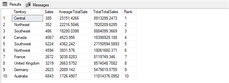
There is a significant difference here in revenue per territory, much more than 5.4%. Territory will be our main predictive variable for how much a customer will spend (in combination with the aforementioned email promotion fact). However, we'll have to encode this information, as described above.
Finally, let's use the IN/SC (individual vs. store) categorization as our third and last predictor.
SELECTp.PersonType,
   COUNT(*) [Sales],
   AVG(h.TotalDue) [AverageTotalSale],
   SUM(h.TotalDue) [TotalTotalSales],
   RANK() OVER ( ORDER BY AVG(h.TotalDue) DESC ) [Rank]
FROM Sales.SalesOrderHeader h
INNER JOIN Sales.Customer c ON h.CustomerID = c.CustomerID
INNER JOIN Person.BusinessEntity b ON c.PersonID = b.BusinessEntityID
INNER JOIN Person.Person p ON b.BusinessEntityID = p.BusinessEntityID
GROUP BY p.PersonType
ORDER BY [Rank]
-- SC = Store Contact, IN = Individual.
-- Great choice here, average for SC is 23850.62 and for IN is 1172.90.
-- Split in terms of quantity is 3806/27659 (around 13% individuals)
We can encode all this data using simple CASE statements (or more complex PIVOT/UNPIVOTs where getting the data is more difficult). Here is a query which will fetch all the data we need, around 31,000 rows.
SELECT CASE p.PersonType WHEN 'SC' THEN 0 ELSE 1 END [PersonType],
   CASE t.[Name] WHEN 'Australia' THEN 1 ELSE 0 END [IsAustralia],
   CASE t.[Name] WHEN 'Canada' THEN 1 ELSE 0 END [IsCanada],
   CASE t.[Name] WHEN 'Central' THEN 1 ELSE 0 END [IsCentral],
   CASE t.[Name] WHEN 'France' THEN 1 ELSE 0 END [IsFrance],
   CASE t.[Name] WHEN 'Germany' THEN 1 ELSE 0 END [IsGermany],
   CASE t.[Name] WHEN 'Northeast' THEN 1 ELSE 0 END [IsNortheast],
   CASE t.[Name] WHEN 'Northwest' THEN 1 ELSE 0 END [IsNorthwest],
   CASE t.[Name] WHEN 'Southeast' THEN 1 ELSE 0 END [IsSoutheast],
   CASE t.[Name] WHEN 'Southwest' THEN 1 ELSE 0 END [IsSouthwest],
   CASE t.[Name] WHEN 'United Kingdom' THEN 1 ELSE 0 END [IsUK],
   CASE WHEN p.EmailPromotion > 0 THEN 1 ELSE 0 END [EmailPromotion],
   h.TotalDue
FROM Sales.SalesOrderHeader h
INNER JOIN Sales.Customer c ON h.CustomerID = c.CustomerID
INNER JOIN Person.BusinessEntity b ON c.PersonID = b.BusinessEntityID
INNER JOIN Person.Person p ON b.BusinessEntityID = p.BusinessEntityID
INNER JOIN Sales.SalesTerritory t ON c.TerritoryID = t.TerritoryID

Now, let's create a new R script in R Studio, and we'll use the 'RODBC' package. This is a package with ODBC connection methods in it, so we can connect easily to our local SQL Server platform. If you haven't yet installed it, install using 'install.packages('RODBC')'. Let's connect to localhost and fetch the results from the query above into a new data frame object.
library(RODBC)
connString = "Driver={Sql Server Native Client 11.0};
      Server=localhost;
      Database=AdventureWorks2016;
      UID=DemoUser;
      PWD=<redacted>"

conn <- odbcDriverConnect(connString)

# A word of warning here - R doesn't take kindly to tabs.
# Make sure you use at least one space between each word.

# Another gotcha - if the user's default DB is not AdventureWorks2016
# the R script can fail due to a bug in the rodbc implementation.
# To cover all eventualities, the 4-part name is used below.
query = "
SELECT TOP 2500
   CASE p.PersonType WHEN 'SC' THEN 0 ELSE 1 END [PersonType],
   CASE t.[Name] WHEN 'Australia' THEN 1 ELSE 0 END [IsAustralia],
   CASE t.[Name] WHEN 'Canada' THEN 1 ELSE 0 END [IsCanada],
   CASE t.[Name] WHEN 'Central' THEN 1 ELSE 0 END [IsCentral],
   CASE t.[Name] WHEN 'France' THEN 1 ELSE 0 END [IsFrance],
   CASE t.[Name] WHEN 'Germany' THEN 1 ELSE 0 END [IsGermany],
   CASE t.[Name] WHEN 'Northeast' THEN 1 ELSE 0 END [IsNortheast],
   CASE t.[Name] WHEN 'Northwest' THEN 1 ELSE 0 END [IsNorthwest],
   CASE t.[Name] WHEN 'Southeast' THEN 1 ELSE 0 END [IsSoutheast],
   CASE t.[Name] WHEN 'Southwest' THEN 1 ELSE 0 END [IsSouthwest],
   CASE t.[Name] WHEN 'United Kingdom' THEN 1 ELSE 0 END [IsUK],
   CASE WHEN p.EmailPromotion > 0 THEN 1 ELSE 0 END [EmailPromotion],
   h.TotalDue
FROM AdventureWorks2016.Sales.SalesOrderHeader h
INNER JOIN AdventureWorks2016.Sales.Customer c ON h.CustomerID = c.CustomerID
INNER JOIN AdventureWorks2016.Person.BusinessEntity b ON c.PersonID = b.BusinessEntityID
INNER JOIN AdventureWorks2016.Person.Person p ON b.BusinessEntityID = p.BusinessEntityID
INNER JOIN AdventureWorks2016.Sales.SalesTerritory t ON c.TerritoryID = t.TerritoryID
ORDER BY ( SELECT NULL )"

importedData <- sqlQuery(conn, query) # save the result set into a data frame object
We have restricted the training set to 2,500 rows. Also, NNs do not cope well with large numerical data. Numerical data ought to be normalized for error calculation to work correctly due to the large ranges possibly skewing the results – by this, we mean the data should be ranged between 0 and 1. We can do this fairly simply – for positive reals, we find the largest value in the column, and for each value in the column, divide it by the largest value to yield a decimal between 0 and 1.
We can see a statistical summary of the data, and view the first few rows of the data, using the summary() and head() methods (write R code in RStudio, or execute as .R file using R.exe):
largest <- max(importedData$TotalDue)
importedData$TotalDue <- (importedData$TotalDue / largest)

summary(importedData)
head(importedData)

Okay, so we've identified our data, encoded it and imported it to our R session as a new in-memory data frame object called importedData.
Building the NN
There are many types of neural network, which behave differently – feedforward, radial basis function (RBF), self-organizing, recurrent, convolutional, back-propagating, modular and so on. Generally, they differ on architecture (back-propagating networks, for example, feedback output into the inputs of predecessor perceptrons) or function type (sigmoid threshold functions, for example, output a different value given an input than a Heaviside step function). The aim of this tip is not to write extensively about these differences, but to make you aware of the varying types of NN – you will find further reading toward the end of this tip. For our purposes, we will create a NN from a predefined library in R called 'neuralnet' – you will find the package documentation in the Next Steps section at the end of this tip. It will be a back-propagating NN which will aim to train itself 100 times (reps), using repeated iterations to reduce the error associated with each weight.
We'll create the NN using the 'neuralnet' package. We will create the NN with 13 inputs (1 input for email promotion, 10 for territory, 2 for customer type as per the columns of our query) and one output (total spend), with 1 hidden layer comprising of 6 neurons. For the error function, we use sum of squared errors (the same function as linear regression) and the default activation function. Bias is random.
Let's append the following code to our R script, using importedData as the data source. If you haven't yet installed package 'neuralnet', run 'install.package('neuralnet')' first. We are using a back-propagating NN with weight adjustments, 6 hidden nodes, the sum of squared errors as the error function, a custom 'softmax' function as the activation (threshold) function, a low error threshold, a relatively high learning rate, 50 training cycles ('epochs') and 2,500 sample rows of data for training purposes. There are many great resources out there for training neural networks – these are just a sample of criteria that may yield an acceptable result.
library(neuralnet)
softmax = custom <- function(x) {log(1+exp(x))}
nn <- neuralnet(importedData$TotalDue ~ # this is the output variable
      importedData$EmailPromotion +        # the following are the independent variablesimportedData$PersonType +
   importedData$IsAustralia +
   importedData$IsCanada +
   importedData$IsCentral +
   importedData$IsFrance +
   importedData$IsGermany +
   importedData$IsNortheast +
   importedData$IsNorthwest +
   importedData$IsSoutheast +
   importedData$IsSouthwest +
   importedData$IsUK,
      data=importedData,       # the name of the data frame
      hidden=6,                # how many neurons do we want in the hidden layer
      err.fct="sse",           # error function: sum of squared errors
   act.fct=softmax,
   algorithm="rprop+",
   threshold=0.05,
   learningrate=0.1,
      linear.output=FALSE,
      rep=50,                   # how many training repetitions for the NN?
   lifesign="full"           # verbose output during training
)
If we run this script, the NN starts training. Depending on the parameters you use, the training may take more or less time due to the level of computation required. Although long training routines can look unwieldy, training the NN is an exercise that can be scripted and scheduled via a stored procedure in SQL Agent to complete on a nightly basis, if necessary (which we will demonstrate towards the end of the tip). Other strategies to reduce this time can include reducing the repetitions, reducing the number of hidden neurons, changing the learning rate, the algorithm or reducing the input data (e.g. by sampling), although these may also reduce the accuracy of the NN.
We can visualize the NN using the plot function. The numbers on each connection are the weights.
plot(nn, rep="best", intercept=0) # We can jazz this up by using parameters to customise the graph.

Testing the NN
The neuralnet package comes with a handy method of testing the reliability of the predictions, using the prediction() method. This method takes the mean of all responses per variable and compares the mean to each response, outputting the error between the two. While this is a valid method it's not ideal for our example, as the variance of outputs (TotalDue) values is very high (thanks in part to having a mix of low- and high-value orders). Therefore, we will use compute() to make predictions against our training data and compare the predicted outputs against the actual outputs instead, working out the difference on a sale-by-sale basis.
# Now the NN is trained, we isolate the independent variables into a new data frame 'indVars':
indVars <- subset(importedData,

select = c( "EmailPromotion","PersonType","IsAustralia","IsCanada","IsCentral","IsFrance",
            "IsGermany","IsNortheast","IsNorthwest","IsSoutheast","IsSouthwest","IsUK"))
head(indVars)
# Now we demonstrate the 'compute' function (in neuralnet), which computes the expected outputs.
nn.results <- compute(nn, indVars)
results <- data.frame(actual=importedData$TotalDue, prediction=nn.results$net.result)
We can now characterize the differences using standard statistical methods – the mean and median average differences and percentile/standard deviation of the same, and approximate an overall percentage – in other words, how accurate (%), on average, is our model at predicting total revenue of a given customer given their status (individual/store), territory and whether or not they arrived via an email promotion?
The output of the NN.compute() function is a list containing each neuron's output for each layer of the network, so all we need is the list of outputs (our output vector) for the output node. These are ordered, so we match them up against the inputs by simply extracting the output vector and appending it as a new column in importedData.
Now, we can calculate the differences by adding a new column into importedData with the values of the differences between importedData$TotalDue and importedData$PredictedTotalDue – a simple subtraction.
comparison <- cbind(importedData$TotalDue, results$prediction)
comparison <- data.frame(comparison)
comparison$X1 <- comparison$X1 * largest
comparison$X2 <- comparison$X2 * largest
comparison$delta <- comparison$X1 - comparison$X2
colnames(comparison) <- c("actual","predicted","delta")
We now need to validate that our NN is answering the question we asked – given some customer details, how much are they likely to spend? We can do this by examining the data. The following plots show the actual amounts spent vs. the predictions made by our NN. You will immediately notice how the predictions are grouped into 20 values. There are a few ways we can assess for accuracy here, but we will keep it simple. We will check the set of predictions against a set of random data and see which set was closest to the actual values, and by how much. This will give us an indication of whether our model is providing any value and allow us to quantify that value.
Let's generate a uniform vector of random values between the lowest and the highest values in the comparison$actual column, and create a second delta column for the differences between the actual values and the random values. We will then lose the sign and both sum and (mean) average the delta column and the random delta column.
comparison <- cbind(comparison$actual, comparison$predicted, comparison$delta, runif(nrow(comparison), min=min(comparison$actual), max=max(comparison$actual)))
comparison <- data.frame(comparison)
colnames(comparison) <- c("actual","predicted","delta","random")
comparison$randomDelta <- comparison$actual - comparison$random
head(comparison)
comparison$delta <- abs(comparison$delta)
comparison$randomDelta <- abs(comparison$randomDelta)
sum(comparison$delta)
sum(comparison$randomDelta)
mean(comparison$delta)
mean(comparison$randomDelta)
This yields:
| Sum | Mean | |
| Prediction Delta | 54598589 | 21839 |
| Random Delta | 195844170 | 78337 |
This is an interesting result – what we're saying, to put it simply, is that on average our prediction is 21,839 off the actual value which, on the face of it, seems poor. However, if we were to choose a random value (from all known values), that random value would, on average, be 78,337 off the actual value. In other words, our model is able to predict the value to a much greater degree of accuracy than a random guess. Likewise, the sum of deltas (differences) for 2,500 records is 54 million for our predictions, but a massive 195 million for a random guess. In other words, our model is more than 4 times more likely to correctly predict (with a moderate margin of error) the amount spent by a customer than a random guess.
This is easier to grasp when visualized. Below are the graphs of the differences between actual amount spent vs. predicted amount spent, and actual amount spent vs. random values. You can see there is much less of an error between the predicted amount and actual amount, far stronger than random amount and actual amount.

Integrating the NN with SQL Server
This is the final section of the tip, in which we integrate our work with SQL Server. We will create a stored procedure that creates and trains a NN from an existing table of data, and which inserts the definition of the NN (metadata) into a metadata table; and a stored procedure that retrieves a NN model from the metadata and makes a prediction, given a full set of input variables.
We can use the RevoScaleR package in R for SQL Server to save our neural network to a VARBINARY(MAX) object and recall it from a table whenever we need it, without retraining the model each time, which is essential if we want to create quick predictions. Create the following table in SQL Server:
USE AdventureWorks2016
CREATE TABLE dbo.NeuralNetworkDefinitions (
    id VARCHAR(200) NOT NULL PRIMARY KEY,
    [value] VARBINARY(MAX) )
Now create a new connection in R and use rxWriteObject to save the model to the table:
connStr <- 'Driver={SQL Server};Server=localhost;Database=AdventureWorks2016;User=DemoUser;Password=<redacted>'
conn <- RxOdbcData(table="NeuralNetworkDefinitions", connectionString=connStr)
rxWriteObject(conn, "<name of model>", nn)
We can retrieve the model from the table into the 'nn' variable using the opposite function:
nn <- rxReadObject(conn, "<name of model>")
Here are the two procedures which will enable us to train a new neural network and use an existing neural network to make predictions. Feel free to amend these to suit your purposes – for example, adding input parameters to reference the data, or by extracting the prediction into a variable, table or return value. Please see the note at the beginning of this tip about Revolution (Revo) components required to use R – if you don’t need to integrate this far with SQL Server, this tip can be used in the context of standalone R scripts called using R.exe (in the bin directory of your R installation), callable using the operating system script component of a SQL Agent job.
CREATE PROCEDURE TrainNewNeuralNetwork
AS BEGIN
   EXEC sp_execute_external_script
      @language = N'R',
      @script = N'
library(RODBC)
library(neuralnet)
connString = "Driver={Sql Server Native Client 11.0};
            Server=localhost;
            Database=AdventureWorks2016;
            User=DemoUser;Password=<redacted>"
conn <- odbcDriverConnect(connString)
query = "
SELECT -- all data this time, not a sample - beware of training times with too many rows
      CASE p.PersonType WHEN 'SC' THEN 0 ELSE 1 END [PersonType],
      CASE t.[Name] WHEN 'Australia' THEN 1 ELSE 0 END [IsAustralia],
      CASE t.[Name] WHEN 'Canada' THEN 1 ELSE 0 END [IsCanada],
      CASE t.[Name] WHEN 'Central' THEN 1 ELSE 0 END [IsCentral],
      CASE t.[Name] WHEN 'France' THEN 1 ELSE 0 END [IsFrance],
      CASE t.[Name] WHEN 'Germany' THEN 1 ELSE 0 END [IsGermany],
      CASE t.[Name] WHEN 'Northeast' THEN 1 ELSE 0 END [IsNortheast],
      CASE t.[Name] WHEN 'Northwest' THEN 1 ELSE 0 END [IsNorthwest],
      CASE t.[Name] WHEN 'Southeast' THEN 1 ELSE 0 END [IsSoutheast],
      CASE t.[Name] WHEN 'Southwest' THEN 1 ELSE 0 END [IsSouthwest],
      CASE t.[Name] WHEN 'United Kingdom' THEN 1 ELSE 0 END [IsUK],
      CASE WHEN p.EmailPromotion > 0 THEN 1 ELSE 0 END [EmailPromotion],
      h.TotalDue
FROM AdventureWorks2016.Sales.SalesOrderHeader h
INNER JOIN AdventureWorks2016.Sales.Customer c ON h.CustomerID = c.CustomerID
INNER JOIN AdventureWorks2016.Person.BusinessEntity b ON c.PersonID = b.BusinessEntityID
INNER JOIN AdventureWorks2016.Person.Person p ON b.BusinessEntityID = p.BusinessEntityID
INNER JOIN AdventureWorks2016.Sales.SalesTerritory t ON c.TerritoryID = t.TerritoryID
"
importedData <- sqlQuery(conn, query) # save the result set into a data frame object
largest <- max(importedData$TotalDue)
importedData$TotalDue <- (importedData$TotalDue / largest)
softmax = custom <- function(x) {log(1+exp(x))}
nn <- neuralnet(importedData$TotalDue ~  # this is the output variable
            importedData$EmailPromotion +      # the following are the independent variables
   importedData$PersonType +
   importedData$IsAustralia +
   importedData$IsCanada +
   importedData$IsCentral +
   importedData$IsFrance +
   importedData$IsGermany +
   importedData$IsNortheast +
   importedData$IsNorthwest +
   importedData$IsSoutheast +
   importedData$IsSouthwest +
   importedData$IsUK,
      data=importedData,    # the name of the data frame
      hidden=6,             # how many neurons do we want in the hidden layer?
      err.fct="sse",        # error function: sum of squared errors
   act.fct=softmax,
   algorithm="rprop+",
   threshold=0.05,
   learningrate=0.1,
      linear.output=FALSE,
      rep=50,               # how many training repetitions for the NN
      lifesign="full"       # verbose output during training
)
connStr <- 'Driver={SQL Server};Server=localhost;Database=AdventureWorks2016;User=DemoUser;Password=<redacted>'
conn <- RxOdbcData(table="NeuralNetworkDefinitions", connectionString=connStr)
rxWriteObject(conn, "NeuralNetwork", nn)'
END
CREATE PROCEDURE MakePredictionWithNeuralNetwork
AS BEGIN
   EXEC sp_execute_external_script
   @language = N'R',
   @inputData1 = 'SELECT 0, 1, 0, 0, 1, 0, 0, 0, 0, 0, 0, 0',
   -- input vars, could also fetch from table or pass as a set of parameters.
   @script = N'
connStr <- 'Driver={SQL Server};Server=localhost;Database=AdventureWorks2016;User=DemoUser;Password=<redacted>'
conn <- RxOdbcData(table="NeuralNetworkDefinitions", connectionString=connStr)
nn <- rxReadObject(conn, "NeuralNetwork")
indVars <- subset(importedData,
      select = c( "EmailPromotion","PersonType","IsAustralia","IsCanada","IsCentral","IsFrance",
      "IsGermany","IsNortheast","IsNorthwest","IsSoutheast","IsSouthwest","IsUK"))
nn.results <- compute(nn, indVars)
results <- data.frame(prediction=nn.results$net.result)
results$prediction '
WITH RESULT SETS (([Prediction] FLOAT));
-- Remember to de-normalise the prediction - multiply by largest available actual sale amount.
END
This process forms the basis for the next step in the business logic – sending the customer through the most appropriate marketing channel; assigning the customer to the most appropriate sales team or agent; or offering the customer a discount or coupon depending on their likely spend.
Next Steps
In summary, we have successfully used SQL Server and R to source customer demographics from AdventureWorks, build a machine learning model (back-propagating neural network) to represent expected revenue per sale, and integrated the model into a stored procedure and function within SQL Server for use by the business.
Please see the links below for more information.
- Siddarth Mehta – Getting Started With R in SQL Server – https://www.mssqltips.com/tutorial/getting-started-with-r-in-sql-server/
- Derek Colley – SQL Server Data Access Using R (Part 1) – https://www.mssqltips.com/sqlservertip/4880/sql-server-data-access-using-r–part-1/
- Vitor Montalvao – Setup R Services for SQL Server 2016 – https://www.mssqltips.com/sqlservertip/4686/setup-r-services-for-sql-server-2016/
- Siddarth Mehta – Basics of Machine Learning With SQL Server 2017 And R – https://www.mssqltips.com/tutorial/basics-of-machine-learning-with-sql-server-2017-and-r/
- R package ‘neuralnet’ Documentation – https://cran.r-project.org/web/packages/neuralnet/neuralnet.pdf
- R package ‘RODBC’ Documentation – https://cran.r-project.org/web/packages/RODBC/RODBC.pdf
- Fitting a Neural Network in R; neuralnet package – https://www.r-bloggers.com/fitting-a-neural-network-in-r-neuralnet-package/
- Microsoft – R Services in SQL Server 2016 – https://docs.microsoft.com/en-us/sql/advanced-analytics/r/sql-server-r-services?view=sql-server-2017
- Quora – Fine-tuning Neural Networks – https://www.quora.com/How-should-one-select-parameters-when-fine-tuning-neural-networks

Dr. Derek Colley is the lead technical consultant for Optimal Computing, a boutique data consultancy based in the UK NW helping clients troubleshoot, configure, plan and deploy their data platforms. He specializes in data integration and database performance optimization, and is a PhD candidate with Staffordshire University, looking into methods of integrating AL query selection algorithms with the cost-based query optimizer. In his spare time, he enjoys building robots, going outdoors, and spending time with his four children.
- MSSQLTips Awards: Trendsetter (25+ tips)