Problem
Many companies are placing their corporate information into data lakes in the cloud. Since storage costs are cheap, the amount of data stored in the lake can easily exceed the amount of data in a relational database. Regardless of the types of files in the data lake, there is always a need to transform the raw data files into refined data files. How can we program and execute data engineering task using Apache Spark?
Solution
Microsoft Azure has two services, Databricks and Synapse, that allow the developer to write a notebook that can execute on a Spark Cluster. Today, we are going to talk about the two design patterns that can be used to take a raw file and transform it into a refined file.
Big Data Concepts
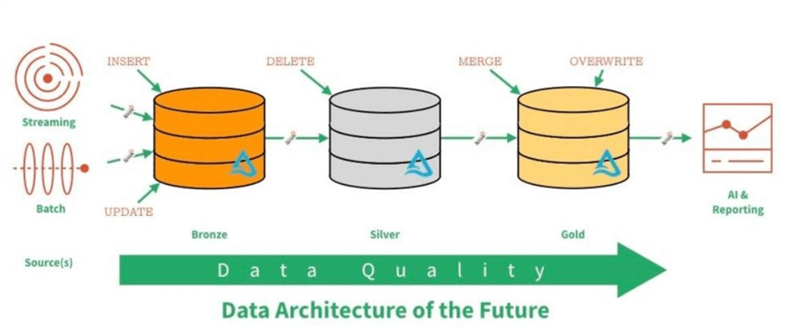
File storage is a key component of any data lake design. The image below depicts a typical lambda architecture. Batch data is usually ingested on a pre-determined schedule. On the other hand, streaming data is processed as soon as information hits the message queue or event hub. The quality of the data increases as you move from one zone to another. Some data architects use the terminology of raw, refine and curated as zones names instead of metals to described quality.
The developer must define the quality zones for the topmost folders for the lake. This can be done by using Azure Storage Explorer. The conventions used for naming of files and folders should contain information about the source system and source category.
The Apache Spark ecosystem allows the data engineer to solve four types of problems: engineering, graph, streaming, and machine learning. In its simplest form, data engineering involves reading up one or more files; combining, cleaning, or aggregating the data in a unique way; and writing out the result to a file in the data lake. The image below shows that both SQL and Dataframes are the two spark technologies that can be used by the developer to solve engineering problems.

This section has gone over the big data concepts of a Data Lake and Apache Spark. Today, we are going explore two design patterns using the Azure Databricks service. The first design pattern uses Spark Dataframes to read up loan club data and write out transformed data. This technique is popular with data scientist who spend a lot of time clean up data with Pandas. The second design pattern uses Spark SQL. This technique is popular with database developers who have been using ANSI SQL for years. Again, the same data is processed two ways but the process ends up with the same result. At the end of the day, we want to publish the refined files as hive tables for easy consumption by the end users.
Loan Club Data
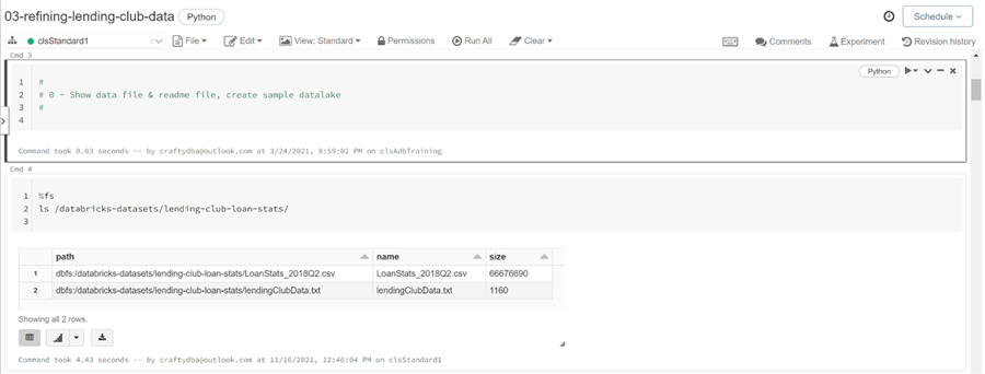
In real life, the Azure Data Lake Storage should be mounted to the Azure Databricks system. This allows for the storage of large amounts of files using the remote storage service. However, there are no sample datasets in a new Azure Storage container. Azure Databricks has local storage that comes with a bunch of sample datasets. These data sets can be used by programmers who are starting to learn Spark programming. The image below shows that two files exist in the “lending club loan stats” folder. Use the file system magic command with the ls sub command to list the files in the directory.
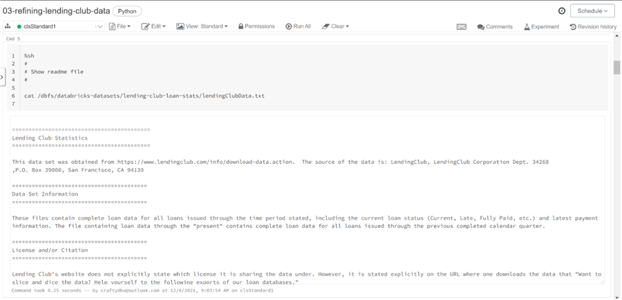
There are several ways to show the contents of a file without using the Spark framework. Use the system shell magic command with the cat sub command to show the contents of the readme file.
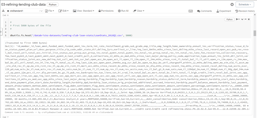
The dbutils library that comes with Databricks contains a bunch of system utilities. Any commands related to the file system can be found under the fs name space. The image below shows the usage of the head function which takes both a fully qualified data file path and total bytes to read as input. Executing the command writes the contents of the file out as output.
Data Engineering – Typical quality zones in a data lake
The notebooks within Azure Databricks system support some of the magic commands that are available within the iPython (Jupyter Notebook) library. Today, we found the source location of the loan club data. Our next task is to create a sample data lake folder structure that can be used with our data engineering patterns.
Sample Data Lake
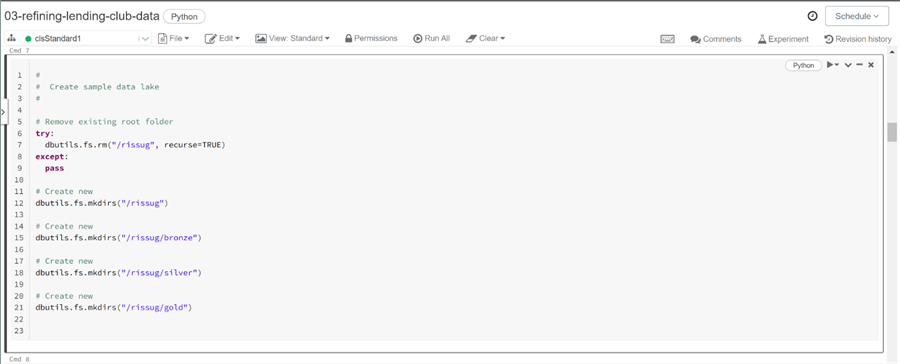
The file system commands in the Databricks utilities library are very helpful. They allow the developer to create and remove both files and directories. The image below shows a simple python code that removes the root directory named RISSUG using the rm command. This acronym stands for the “Rhode Island SQL Server User Group”. I have been involved in this local group since 2009. The rest of the script creates each of the quality zones directory as well as the root directory. These tasks are accomplished using the mkdirs command.
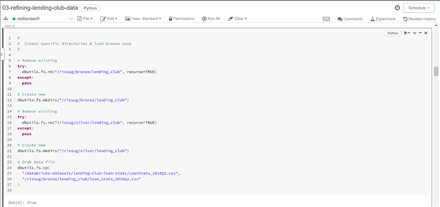
The next step is to create a business specific directory under each of the quality zones that we are using. The code below creates the lending_club directory and copies over the sample data file into the bronze quality zone.
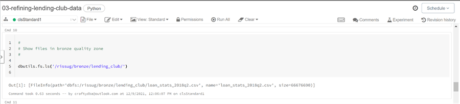
To verify the existence of the source file, we can use the ls command from the Databricks utility library. The function returns an array of FileInfo objects.
The management of files and directories is a key concept when working with a data lake system. Please see my prior article that has more details on this topic.
Spark – Read & Write
Regardless of the design pattern, the spark library has two key functions: read and write. There are a variety of options that can be specified when calling these functions. Please look at the online documentation for details. The python code below reads a comma separated values file into a data frame. The header option tells the underlying Scala code in the Spark Engine to ignore the first line as data. The display command outputs the rows of data into a grid for the user to view. The nice thing about Azure Databrick Notebooks is the ability to turn the grid output into a graph by clicking a button.
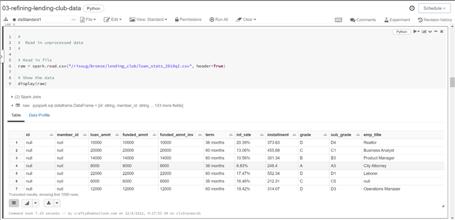
The above image depicts the wideness of the Spark DataFrame for the loan file. There are 143 columns in loan club statistics file. This is quite typical in commercial off the shelf (COTS) packages. For easier consumption, the data architect will pare down this list to key columns that will be used by the end users.
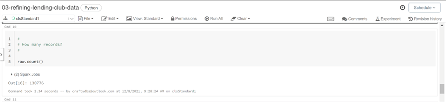
Many developers use record and column counts as a quick assertion (sanity check) that a data processing job completed successfully. The count method of the Spark DataFrame shows the loan dataset having around 131 K rows.
Dataframe Processing
The first design pattern uses the fact that the Spark DataFrame has methods that can be used to transform the data from one form to another. The number of methods for Spark DataFrame is too numerous to cover in this article. Please use the hyperlink to research the different ways you can transform data.
The following algorithm was used to clean up the loan club statistics data set.
| Step | Description |
|---|---|
| 1 | Reduce the number of columns in the final dataset. |
| 2 | Create derived column called [bad loan]. |
| 3 | Convert [int rate] column from string to float. |
| 4 | Convert [rev util] column from string to float. |
| 5 | Convert [issue year] column from string to double. |
| 6 | Convert [earliest year] column from string to double. |
| 7 | Created derived column [credit length in years] from previous two columns. |
| 8 | Clean up [emp length] column using regex expression and convert to float. |
The following python code transforms the data stored in the raw variable. The results of data processing is a variable named loans1. This variable is written out to a parquet file that is partitioned into two files. Partition is very important when processing large datasets using a big cluster.
#
#  Design Pattern 1 - Process data via dataframe commands
#
# Include functions
from pyspark.sql.functions import *
# Choose subset of data
loans1 = raw.select(
  "loan_status",
  "int_rate",
  "revol_util",
  "issue_d",
  "earliest_cr_line",
  "emp_length",
  "verification_status",
  "total_pymnt",
  "loan_amnt",
  "grade",
  "annual_inc",
  "dti",
  "addr_state",
  "term",
  "home_ownership",
  "purpose",
  "application_type",
  "delinq_2yrs",
  "total_acc"
)
# Create bad loan flag
loans1 = loans1.withColumn("bad_loan", (~loans1.loan_status.isin(["Current", "Fully Paid"])).cast("string"))
# Convert to number (int rate)
loans1 = loans1.withColumn('int_rate', regexp_replace('int_rate', '%', '').cast('float'))
# Convert to number (revolving util)
loans1 = loans1.withColumn('revol_util', regexp_replace('revol_util', '%', '').cast('float'))
# Convert to number (issue year)
loans1 = loans1.withColumn('issue_year',  substring(loans1.issue_d, 5, 4).cast('double') )
# Convert to number (earliest year)
loans1 = loans1.withColumn('earliest_year', substring(loans1.earliest_cr_line, 5, 4).cast('double'))
# Calculate len in yrs
loans1 = loans1.withColumn('credit_length_in_years', (loans1.issue_year - loans1.earliest_year))
# Use regex to clean up
loans1 = loans1.withColumn('emp_length', trim(regexp_replace(loans1.emp_length, "([ ]*+[a-zA-Z].*)|(n/a)", "") ))
loans1 = loans1.withColumn('emp_length', trim(regexp_replace(loans1.emp_length, "< 1", "0") ))
loans1 = loans1.withColumn('emp_length', trim(regexp_replace(loans1.emp_length, "10\\+", "10") ).cast('float'))
# Show the data
display(loans1)
# Write out data (force)
loans1.repartition(2).write.mode("overwrite").parquet('/rissug/silver/lending_club/process01.parquet')
The following table lists the methods that were used to transform the DataFrame. I suggest you read about how each method works and how the python code transforms the raw data.
| No | Method | Purpose |
|---|---|---|
| 1 | select | Reduce the number of columns in the dataframe. |
| 2 | withcolumn | Create new or modify existing column. |
| 3 | isin | Compare variable to members in set for matching. |
| 4 | cast | Change the data type of the column. |
| 5 | substring | Return a portion of a string. |
| 6 | trim | Remove white space before and after. |
| 7 | regexp_replace | Perform string manipulation using regular expressions. |
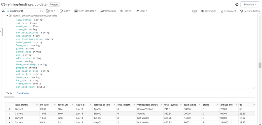
The image below shows the first records of the processed dataframe. We can see the number of columns is considerably smaller. If you are curious, examine the derived and modified columns. These columns contain the lion share of the spark programming code.
Regardless of design pattern, the use of read and write methods of the spark library are always part of a data engineering notebook.
Hive Tables
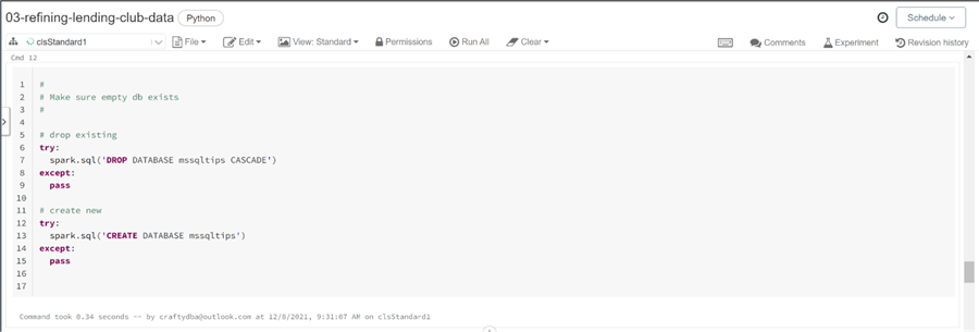
The easiest way to present data to the end users is to create a hive table. Before you can create a table, we must have a hive database. We can always use the default database; however, I like to name my databases after the data they contain. The code below uses spark.sql to execute database commands. If the mssqltips database exists, it is dropped, otherwise a new database is created.
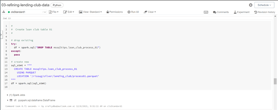
Typically, I drop and recreate the definition of the hive table. The first command below tries to drop the table. The second command below creates an unmanaged table named loan_club_process_01.
What is the difference between managed and unmanaged tables? A managed table is created by specifying the structure of the table and loading the table with an insert statement. The create table as syntax will also create a managed table. Such tables are stored with the hive catalog. Deleting the hive table results in deleting the data (delta files). An unmanaged table uses the location parameter to specify where the underlying file(s) are stored. Dropping the table does not result in the deleting of the files from the storage system.
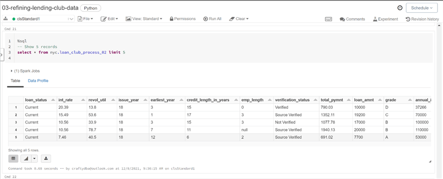
Why did we go thru the effort of creating a hive table for the resulting loan club statistics file? Because the end users can query the file just like a table. The image below shows the first five records of the table named loan_club_process_01.
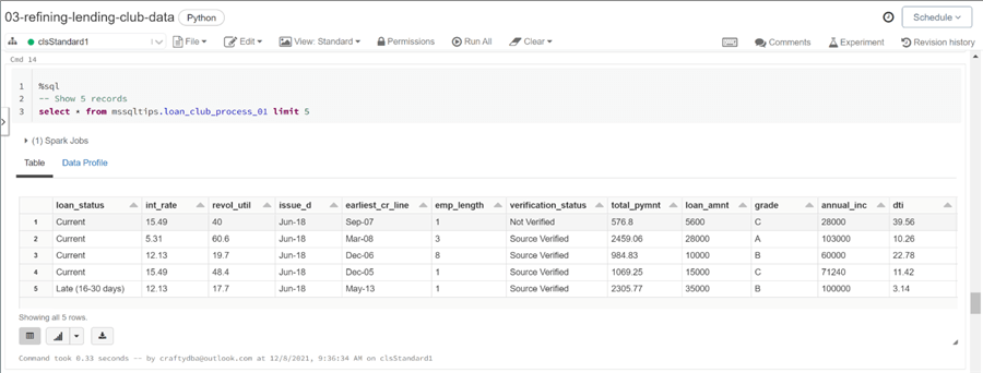
In a nutshell, the hive catalog is a real easy way to expose the underlying files to the end users. Any users who are familiar with ANSI SQL will be right at home with querying the data. I hope you are not surprised by the fact that Spark SQL is the second design pattern that we are going to talk about next.
SQL Processing
The second design pattern uses the fact that a temporary view can be created off any Spark DataFrame. The image below shows the view named tmp_loan_club being created from the Spark DataFrame named raw. The createOrReplaceTempView method is key to this pattern.
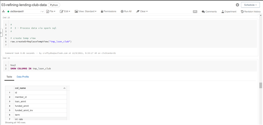
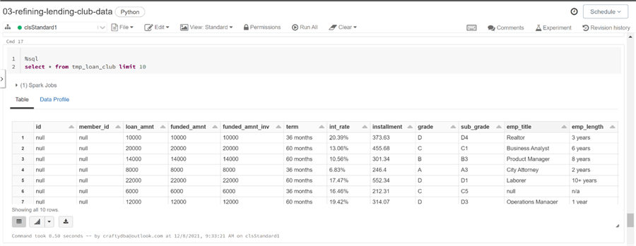
The SHOW COLUMNS command in Spark SQL is very useful when you have a wide hive table and you want to search for a particular name. The image below shows a simple SELECT statement that returns the first ten rows of the table.
The processing algorithm is completely the same as the first design pattern. In fact, there is almost a one to one replace of DataFrame methods with Spark SQL Functions. Please review the on-line documentation for complete details on all supported functions. The only noticeable coding different is the replacement of the isin set operator with a case clause.
#
#  Design Pattern 2 - Process data via Spark SQL code
#
# Multi line here doc
sql_stmt = """
select
  loan_status,
  cast(regexp_replace(int_rate, '%', '') as float) as int_rate,
  cast(regexp_replace(revol_util, '%', '') as float) as revol_util,
  cast(substring(issue_d, 5, 4) as double) as issue_year,
  cast(substring(earliest_cr_line, 5, 4) as double) as earliest_year,
  cast(substring(issue_d, 5, 4) as double) -
  cast(substring(earliest_cr_line, 5, 4) as double) as credit_length_in_years,
  cast(regexp_replace(regexp_replace(regexp_replace(emp_length,
    "([ ]*+[a-zA-Z].*)|(n/a)", ""), "< 1", "0"), "10\\+", "10") as float) as emp_length,
  verification_status,
  total_pymnt,
  loan_amnt,
  grade,
  annual_inc,
  dti,
  addr_state,
  term,
  home_ownership,
  purpose,
  application_type,
  delinq_2yrs,
  total_acc,
  case
    when loan_status = "Current" then "false"
    when loan_status = "Fully Paid" then "false"
    else "true"
  end as bad_loan
from
  tmp_loan_club
"""
# Run spark sql & retrieve resulting df
loans2 = spark.sql(sql_stmt)
# Write out data
loans2.repartition(2).write.mode("overwrite").parquet('/rissug/silver/lending_club/process02.parquet')
When developing the Spark SQL, I usually query the temporary table interactively until I get the output looking exactly like I want. Next, I copy the Spark SQL into a here document, multi-line string that starts and ends with a triple instance of quotes. The last two lines of the program can be described as the following: save the results of a query to a dataframe and write the resulting dataframe to parquet file that has been partitioned into two.
Both the DataFrame processing (pattern 1) and SQL processing (pattern 2) design patterns end up with the same results. I like using the pattern 2 since many clients are very familiar with ANSI SQL. This means the learning curve for an IT professional to become productive is lower than pattern 1.
Querying Hive Tables
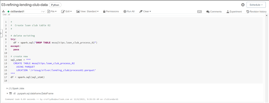
Just like the first design pattern, we want to recreate a hive table given the location of the output file for the second design pattern. To test the results, we can execute a SELECT statement that returns the first five rows of the table named loan_club_process_02.
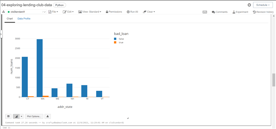
The Spark SQL queries we have used so far are quite simple in nature. The query below aggregates loan data by state name and loan status. Only loans in the New England states are shown. The count of loans and average amount of each loan by grouping criteria is shown.
%sql
select
  addr_state,
  bad_loan,
  count(loan_amnt) as num_loans,
  round(avg(loan_amnt), 4) as avg_amount
from
  mssqltips.loan_club_process_02
where
  addr_state in ('RI', 'CT', 'MA', 'NH', 'VT', 'ME')
group by
  addr_state,
  bad_loan
having
  count(loan_amnt) > 0
order by
  addr_state,
  bad_loan
One of the cool things about Databricks is the fact that charting can be done directly from an output grid. The bar chart below shows that Massachusetts has the largest number of loans for the lending club.
The ability to place a hive table structure on top of a file makes the Spark ecosystem very attractive for data processing. Today, we demonstrated how to read, transform, and write data. More complex processing logic can be created with the saving of intermediate steps to temporary files and exposing those files to down stream processing using temporary views.
Summary
Apache Spark is gaining wide acceptance as an ecosystem that can solve data, graph, machine learning and streaming problems. Big data processing can be achieved by splitting the data into partitions and creating a cluster that has enough cores (slots) to process the data in parallel. Optimization of the storage and programming is key to efficient processing.
Today, we talked about two ways to execute data engineering notebooks. Both techniques must read (extract) and write (load) using Spark DataFrame. The key difference is which method will you choose to perform the translation of the data?
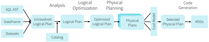
The above image shows how the spark engine reads in notebook code, generates logical plans, picks a physical plan by using a cost optimizer and creates Java Byte code that can be executed by the nodes of the cluster. It is very important to note that both SQL and DataFrame code is translated by the same engine into the similar code.
My closing remark is the following, unless you really want to learn all the methods of the Apache Spark DataFrame, I suggest you leverage your existing SQL skills in this exciting new area of work. Use this link to download the python program for data engineering and accompanying Spark SQL query for reporting.
Next Steps
- Install and use community Python libraries to solve real world problems
- How to read and write efficiently to a SQL Server database
- Going back in time with delta tables

John Miner is a Senior Data Architect at Insight Digital Innovation helping corporations solve their business needs with various data platform solutions.
He has over thirty years of data processing experience, and his architecture expertise encompasses all phases of the software project life cycle, including design, development, implementation, and maintenance of systems.
His credentials include undergraduate and graduate degrees in Computer Science from the University of Rhode Island. Also, he has earned certificates from Microsoft for Database Administration (MCDBA), System Administration (MCSA), Data Management & Analytics (MCSE), Data Science (MPP), Databricks Certified, and Fabric Certified.
John has been recognized with the Microsoft MVP award nine times for his outstanding contributions to the Data Platform community.
When he is not busy talking to local user groups or writing blog entries on new technology, he spends time with his wife and daughter enjoying outdoor activities. Some of John’s hobbies include wood working projects, crafting a good beer and playing a game of chess.
- MSSQLTips Awards: Author of the Year – 2019, 2022, 2023 | Champion (100+tips) – 2023