Problem
The management of data in a relational database eventually boils down to CPU, RAM, and DISK. Since the DISK subsystem is the slowest component in any computer design, it is important to optimize the number of pathways to the storage device. Operations such as a full table scan have to traverse all data pages in a table to obtain the final result. The time spent for such an operation increases as the size of the data increases. How can we decrease the execution time of normal queries and/or database maintenance?
Solution
Some popular ways in SQL Server to partition data are database sharding, partitioned views and table partitioning. The technique divides the data into buckets using some type of hash key such as a date and/or a natural key. By placing the partitions on different files, database parallelism can be increased and the execution time reduced.
Typically, deleting data is a time-consuming effort since all data pages of a given table have to be searched given the delete criteria. When using partitioning, we are dealing with logical objects such as a table, file group and file. The time to delete this meta-data is extremely quick. Finally, backup operations can be simplified since most companies do not rewrite history. Thus, if we are partitioning data by quarters of a year, older logical objects can be backed up once and set to read-only.
Business Problem
The Big John’s BBQ company was established in 2011. The goal of the company is to send out packages of pig parts to members on a monthly basis. Internal users of the company website have been complaining that the latency of the system has been increasing over time. Because users hardly search for data that is more than three months old, the main customer table is a great candidate for partitioning.
Today, we are going to migrate data from the current datamart (warehouse) to a new database that uses a partitioned view. The goal is to reduce the execution time of queries while not impacting the current software.
Current Database Design
It is always best to know what your client does for a living. That way, you can provide the right solution with the correct budget. The image below shows the parts of a pig that you might see in a grocery store. In my spare time, I love making smoked pulled pork using the butt of a pig.

The database for Big John’s BBQ has two dimension tables and one fact table. It was purposely created this way since we want to focus on the technique, not a complex database schema. The query below uses the system catalog views to return detailed information about the database schema.
--
-- Q1 - Find database objects
--

select
  s.name, o.name, o.type_desc
from
  sys.objects o join sys.schemas s
on
  o.schema_id = s.schema_id
where
  is_ms_shipped = 0 and s.name in ('DIM', 'FACT')
order by
  o.type;
The screen shot below was taken from SQL Server Management Studio (SSMS). It shows 14 user defined objects. The last three objects are of real importance since they store the data.

Many times, the table with the largest number of records is the only one that needs attention. In our case, we are looking to reduce query time on the CUSTOMERS table in the FACT schema. The execution of the COUNT function is one way to get record counts by table name. However, this may take considerable time with larger tables. A quicker way to retrieve the same result is to grab the extended object property of the table using the OBJECTPROPERTYEX function.
--
-- Q2 – Grab table counts
--

select
  s.name as the_schema_name,
  t.name as the_table_name,
  OBJECTPROPERTYEX(t.object_id, 'Cardinality') as the_row_count
from
  sys.tables t join sys.schemas s
on
  t.schema_id = s.schema_id
where
  is_ms_shipped = 0 and s.name in ('DIM', 'FACT');
The above snippet shows T-SQL code to return the schema name, table name and row count for all tables in the current database. The below image shows results of executing the query. We can see that the CUSTOMERS table has almost 1 million records.

Many things in the SQL Server engine have changed over time. However, the basic engineering diagram is shown below. Any user defined database usually has one log file and one or more data files. Increasing the number of data files increases the potential IOPS for the database server. Of course once you solve one bottleneck, another one will crop up to limit performance.

Before we start creating a new database for the partitioned view, we should look at the number of files and filegroups in the existing database. The image below shows that there is one data and one log file in the BIG_JONS_BBQ_DW database.
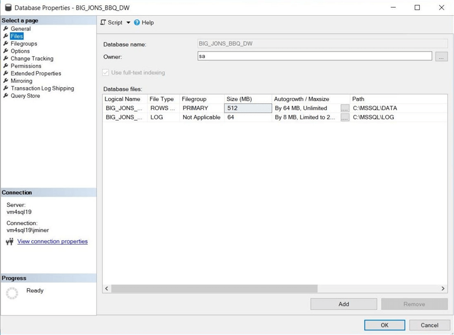
By default, all objects are stored in the PRIMARY file group. This includes all the system tables and views. This database does not have any user defined filegroups.

To recap, the current database has one table that has almost 1 million rows. We want to create a partitioned view to decrease the execution time of queries without significant changes to the front-end website code.
New Database Design
The new database design can be designed in two pieces. First, the static dimensional data in the date and pig packages tables can be brought over as is since the volume of the data is quite low. Also, the function to create hash keys can be coded and deployed to the DIM schema. Second, the dynamic fact data is where partitioning is needed to increase performance and reduce the maintenance burden of the customers table. Let’s work on the first static piece now.
The image below shows a new database named BBQ_PART_VIEW has been created on SQL Server 2019 within an Azure VM named vm4sql19.

The use of schemas is very powerful since we can assign security at this container level. We will be creating a schema for both the static data (DIM) and the dynamic data (FACT). The image below shows the existence of these two new schemas.

At this point, we do not have any tables in the BBQ_PART_VIEW database. We want to create the two new tables in the DIM schema and load them with data from the BIG_JONS_BBQ_DW database.

The above image shows an empty database with no tables. The below image shows the output from the T-SQL script which is enclosed here. Please execute queries 1 to 8 to catch up with the article.

If we run the T-SQL script below, we will list the objects defined in the new database and count their occurrences.
--
-- Q3 – Grab table counts
--

select
  o.type_desc as object_type,
  COUNT(*) as object_count
from
  sys.objects o join sys.schemas s
on
  o.schema_id = s.schema_id
where
  is_ms_shipped = 0 and s.name in ('DIM', 'FACT')
group by
  o.type_desc
order by
  o.type_desc;
Looking at the image below, I was expecting two tables, each with a primary key constraint. However, we have an additional object. Why is there a scalar function?

The scalar function is used to convert a date string to an integer hash that will be used in partitioning of the data. This function does not belong to the FACT schema since we might want to drop and rebuild this schema at any time during testing. The code below looks up the date string in the date dimension table and returns integers for both the year and quarter. It combines the year and quarter information into a 7-digit hash key.
--
-- 5 - Create user defined functions
--

-- Make a year + quarter hash
CREATE FUNCTION [DIM].[UFN_GET_DATE_HASH] (@VAR_DATE_STR VARCHAR(10))
  RETURNS INT
BEGIN
  RETURN
  (
    SELECT [date_int_yyyy] * 1000 + [date_int_qtr]
    FROM [DIM].[DIM_DATE] WHERE [date_string] = @VAR_DATE_STR
  )
END;
Now that the static tables have been dealt with, we can move onto the dynamic customers table.
Partitioned View
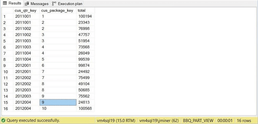
The idea behind a partitioned view is to have the data bucketed by the hash key into separate tables. This eases the management of the data. However, it does not increase the IOPs. Instead of placing all the tables into the default file group and default data file, we want to place each table on its own file group and data file. The image below shows the CUSTOMER data has been partitioned into 4 quarters of data for two years.

The code to dynamically create data files, create file groups, create tables, and insert data is part of one big while loop. However, I did a printout of the first set of commands that we are using to create the objects in the first partition. The code below alters the database to add a new file group called FG_PART_VIEW_2011001 and a new file called FN_PART_VIEW_2011001.
--
-- 9.1 – Modify database
--

-- Add file group
ALTER DATABASE [BBQ_PART_VIEW] ADD FILEGROUP [FG_PART_VIEW_2011001];

-- Add secondary data file to group
ALTER DATABASE [BBQ_PART_VIEW] ADD FILE
(
  NAME=FN_PART_VIEW_2011001,
  FILENAME='C:\MSSQL\DATA\FN_PART_VIEW_2011001.NDF',
  SIZE=16MB, FILEGROWTH=4MB
) TO FILEGROUP [FG_PART_VIEW_2011001];
Using SQL Server Management Studio, we can run a query against catalog views named sys.filegroups and sys.master_files to see our newly created objects. Please remember there is one additional file group named PRIMARY and there are default LOG/DATA files. The image below shows the system data after creating 8 new tables.

The below code adds a table to the new file group.
--
-- 9.2 – Create a new table
--

CREATE TABLE [FACT].[CUSTOMERS_2011001]
(
  cus_id int not null,
  cus_lname varchar(40),
  cus_fname varchar(40),
  cus_phone char(12),
  cus_address varchar(40),
  cus_city varchar(20),
  cus_state char(2),
  cus_zip char(5) not null,
  cus_package_key int not null,
  cus_start_date_key int not null,
  cus_end_date_key int not null,
  cus_date_str varchar(10) not null,
  cus_qtr_key int not null
)
ON [FG_PART_VIEW_2011001];
Finally, we need to add constraints to the newly built table.
--
-- 9.3 – Add constraints to new table.
--

-- Check / Default values
ALTER TABLE [FACT].[CUSTOMERS_2011001] ADD CONSTRAINT CHK_QTR_2011001_KEY CHECK (cus_qtr_key = 2011001);
ALTER TABLE [FACT].[CUSTOMERS_2011001] ADD CONSTRAINT DF_START_2011001_DTE DEFAULT (1) FOR [cus_start_date_key];
ALTER TABLE [FACT].[CUSTOMERS_2011001] ADD CONSTRAINT DF_END_2011001_DTE DEFAULT (365) FOR [cus_end_date_key];

-- Primary / Foreign keys
ALTER TABLE [FACT].[CUSTOMERS_2011001] ADD CONSTRAINT PK_CUST_2011001_ID PRIMARY KEY CLUSTERED (cus_id, cus_qtr_key);
ALTER TABLE [FACT].[CUSTOMERS_2011001] ADD CONSTRAINT FK_DIM_PIG_2011001_PKGS FOREIGN KEY (cus_package_key) REFERENCES [DIM].[PIG_PACKAGES] (pkg_id);
ALTER TABLE [FACT].[CUSTOMERS_2011001] ADD CONSTRAINT FK_DIM_START_2011001_DTE FOREIGN KEY (cus_start_date_key) REFERENCES [DIM].[DIM_DATE] (date_key);
ALTER TABLE [FACT].[CUSTOMERS_2011001] ADD CONSTRAINT FK_DIM_END_2011001_DTE FOREIGN KEY (cus_end_date_key) REFERENCES [DIM].[DIM_DATE] (date_key);
Executing the system query for the prior section that counts objects, we can see that the objects associated with the table are duplicated eight times. Therefore, we have one times eight check constraints. The math continues for each type of constraint.

The code snippet below moves data from the existing database to the new one.
--
-- 9.4 – Move data from existing to new database
--

INSERT INTO [FACT].[CUSTOMERS_2011001]
SELECT * FROM [BIG_JONS_BBQ_DW].[FACT].[CUSTOMERS]
WHERE [CUS_QTR_KEY] = '2011001';
The last step is to create the partitioned view. Here are some rules that must be followed for the query optimizer to work its magic:
- Must use CHECK constraint on hash column
- Primary key must include hash column which can be last item in the list to improve selectivity
- View is created joining multiple tables with a UNION ALL with SCHEMA BINDING
- Tables can be local or distributed
- Insert, update, and delete actions use the same rules as views
The cool thing about partitioned views is that you can add or remove columns from the base tables. You can place default values in the query that the view is based upon for missing data. The query that makes up the view has a limit of 4096 columns in the SELECT statement per documentation. The actual TSQL string can be 64 k times the TDS packet size. Please see this link for database engine limitations.
To summarize this chapter, partitioning of data is achieved by creating a new data file, file group and user table. The hash key has to be part of the primary key for the query optimizer to know which table to query. The view may contain many tables that are schema bound to the definition. I suggest using dynamic T-SQL to create the view since it might be quite lengthy in size.
Please execute queries 9 and 10 in the enclosed T-SQL script to catch up with the article.
Testing SELECT queries
How do we know that the query performance of the new CUSTOMER partitioned view is greater than the old CUSTOMER table? The best way is to execute queries, look at the execution plans and collect timings. The query below gets records counts by quarter hash key.
--
-- Q4 – Get record counts by quarter
--

SELECT
  c.cus_qtr_key,
  count(*) as cus_total
FROM
  [FACT].[CUSTOMERS] c
GROUP BY
  c.cus_qtr_key
ORDER BY
  c.cus_qtr_key;
The execution of this query on the original table takes 1 minute and 51 seconds.

The hash key is part of the primary key in the original table. The query executor spends most of the time scanning a clustered index and performing a hash match aggregate. There is only one execution stream.

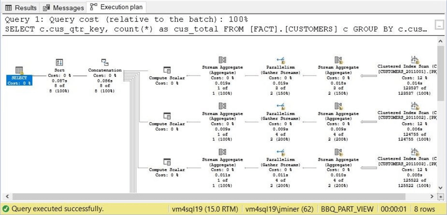
The execution of this query on the new partitioned view takes 1 second.

The hash key is part of the primary key in all the table partitions. The query executor produces a similar clustered index scan and aggregation. However, eight execution streams are created, and the results are concatenated into one result set. In short, the parallelism of this plan with multiple pathways to the disk due to multiple files reduces the execution time to a fraction of original design.
Maybe you are not believing the results at this time. Let us try another query in which additional data that is not part of the primary key is used to calculate the final results.
--
-- Q5 – Get record counts by quarter and package sold
--

SELECT
  c.cus_qtr_key,
  c.cus_package_key,
  count(*) as cus_total
FROM
  [FACT].[CUSTOMERS] c
GROUP BY
  c.cus_qtr_key,
  c.cus_package_key
ORDER BY
  c.cus_qtr_key,
  c.cus_package_key;
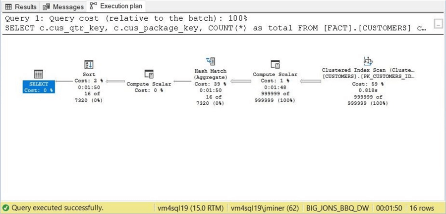
The execution of this query on the original table takes 1 minute and 50 seconds. Can you guess why we have a constant execution time?
The amount of time to scan the table is a constant value. We have a similar execution plan to query named Q4.
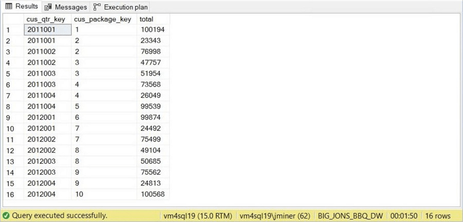
The execution of this query on the new partitioned view takes 1 second. One last chance to guess at the reason behind this similar result.
Again, we end up with a parallel plan that reads from multiple files at the same time. Even though my virtual machine is in the Azure Cloud, we are traversing a million rows and returning the result set back within 1 second.

I hope I sold you on the fact that partitioned views can significantly reduce the execution time of data that is stored in one table and one file.
Testing DELETE queries
Even with reporting systems, business users only want to look at a limited window of data. For instance, year over year reporting is very common in many companies. That means, we might have to remove data from our large table if we are keeping a rolling 24 months of data.
During testing, you might want to make a copy of your data. How can we do this with the original database named BIG_JONS_BBQ_DW? The first step is to take the database offline. This can be done via SQL Server Management Studio.

The next step is to make a copy of both the data and logs files. Since we are duplicating the original database, there is one file of each type. The image below shows the results of a file search using window explorer. The new files have a number 2 at the end of the file name.

You might not know that the CREATE DATABASE command has a syntax that allows you to attach files as a new database. Execute the command below to create the duplicate database.
--
-- Q6 – Create new database from existing data/log files
--

CREATE DATABASE [BIG_JONS_BBQ_DW2] ON
(FILENAME = 'C:\MSSQL\DATA\BIG_JONS_BBQ_DW2.mdf'),
(FILENAME = 'C:\MSSQL\LOG\BIG_JONS_BBQ_DW2.ldf')
FOR ATTACH;
The image below shows the new database copy is online. This is the database that we will be running our DELETE query against.

The TSQL code shown below is the typical way to delete data. For very large tables, we might want to do this action in a loop that limits the number of records and does a checkpoint.
--
-- Q7 – Delete records from one big table
--

DELETE
FROM [FACT].[CUSTOMERS]
WHERE cus_qtr_key = 2011001
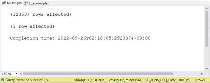
The screen shot below shows the delete action removed 124,537 rows. Again, the execution plan was a clustered index scan that took 1 minute and 50 seconds.
The actual code that removes one quarter of data from the partition view is quite different. Here are the actions that need to be performed.
- Update view by removing one select query from union all.
- Drop existing table for oldest quarter.
- Drop existing file for oldest quarter.
- Drop existing file group for oldest quarter.
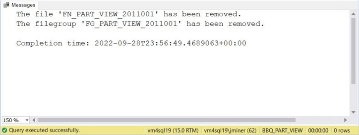
The image below shows that these steps take less than 1 second to execute. That is because all actions are meta data related.
So far, we have seen that both SELECT and DELETE actions that normally take a long time with a large table run faster when the data is organized by a partitioned view.
Summary
With today’s explosion of data, the amount of data stored in your reporting table has increased over time. If you are not bench marking your database daily with a tool, you might not realize that the execution time of the canned and ad-hoc queries have slowed over time. Partitioning is a technique that reduces the access time by bucketing the data into smaller segments that can be searched faster. At the same time, maintenance activities such as backups can be sped up by marking files as read only.
In this article, we reviewed the technique of a partitioned view. A new file, file group and table were created for each partition or hash key. The data was moved from the old reporting system to the new using the hash key in the where clause during insertion. At the end, a partitioned view was used to bind all the tables together as one logical unit. Since this technique uses a view, the limitations of a view apply. For instance, we can’t execute an INSERT statement with data from two partitions to complete successfully. However, executing an INSERT or UPDATE or DELETE statement with data for one partition works fine. To logically remove a partition, we remove the objects in reverse order. Thus, a table, file group and file are DROPPED. However, since the view uses schema binding, we need to update the SELECT query first.
Does the technique of a partitioned view still apply today with table partitioning being mainstream in all editions? I think the answer to this question is YES.
Azure SQL Managed Instance has two flavors: general-purpose and business critical. The general-purpose tier is based upon remote storage. Larger the file, the more IOPS for the database. However, we are capped at 16 TB of disk space for the whole service. Therefore, we do not want a lot of small files that normal table partitioning might create. We want to create larger data files for higher IOPS. For instance, if we create two secondary data files that are over one terabyte in size, we get 7500 IOPS per file. In the example above, we can place 4 tables on a given file. This still gives us the benefit of working with meta-data when DELETING data and parallelism on SELECT queries. I have not tried this out in real life, but it might be a great idea for an article!
As promised, here is the T-SQL used in my normal partitioned view presentation. Any additional T-SQL used for demonstrations in this article can be found in this file.
Next Steps
Check out these related articles:

John Miner is a Senior Data Architect at Insight Digital Innovation helping corporations solve their business needs with various data platform solutions.
He has over thirty years of data processing experience, and his architecture expertise encompasses all phases of the software project life cycle, including design, development, implementation, and maintenance of systems.
His credentials include undergraduate and graduate degrees in Computer Science from the University of Rhode Island. Also, he has earned certificates from Microsoft for Database Administration (MCDBA), System Administration (MCSA), Data Management & Analytics (MCSE), Data Science (MPP), Databricks Certified, and Fabric Certified.
John has been recognized with the Microsoft MVP award nine times for his outstanding contributions to the Data Platform community.
When he is not busy talking to local user groups or writing blog entries on new technology, he spends time with his wife and daughter enjoying outdoor activities. Some of John’s hobbies include wood working projects, crafting a good beer and playing a game of chess.
- MSSQLTips Awards: Author of the Year – 2019, 2022, 2023 | Champion (100+tips) – 2023

Dear Paul White,
First, your database tuning skills rock. I have read many of your articles. I did leave the non performant computed column as non persisted as kind of an Easter Egg. This article is part of a larger deck that I do on effective data warehousing techniques that focus on partitioning. You are the first one to point this out before I asked “what is wrong with this table”. Kudos on your investigational skills.
Second, the purpose of the article is to have people think about how partitioning can reduce maintenance, speed up delete actions and increase query performance by reducing the amount of data you need to search.
Third, many of low end the Platform As A Service offerings do not even have the IOPS that our laptops have. Therefore, tuning and partitioning will play an important role.
Again, thanks for reading my article and your feed back. I will be presenting at PASS in November and hope to bump into you.
Sincerely
John Miner
The Crafty DBA
Data Platform MVP
Hi John,
The big performance problem with the original database (which I downloaded from a link on your blog) was the non-persisted scalar function performing data access per row (with a less than ideal supporting index, as an aside).
The scalar function also prevents all parallelism, even if the computed column is not used in a query against the table.
Replacing the existing computed column with a persisted computed column that doesn’t use a scalar function reduced the execution time from 47 seconds (with actual plan enabled) on my laptop to 64ms (with database compatibility set to 150) in a single-threaded execution plan.
Complete change script:
ALTER TABLE FACT.CUSTOMERS
DROP COLUMN cus_qtr_key;
ALTER TABLE FACT.CUSTOMERS
ADD cus_qtr_key AS
YEAR(TRY_CONVERT(date, cus_date_str, 120)) * 1000 +
DATEPART(QUARTER, TRY_CONVERT(date, cus_date_str, 120))
PERSISTED;
ALTER TABLE FACT.CUSTOMERS
REBUILD WITH (MAXDOP = 1);
Cheers,
Paul
Hi Dmitry,
I am ecstatic that you enjoyed the article. I write to teach people new techniques or refresh old ones.
As for your question, we partitioned by a hash key (yyyy qqq). If you use the hash key in your query, it will be guaranteed to select the correct table.
If you decide to query by a date key not date since it is a dimension model, it will have to search all eight tables. However, the search is done in parallel using a clustered index scan. Thus, it will perform better than a single table scan in the original design.
If date is truly important for querying, you can use it as the hash key; However, the number of tables will increase. At least 365 per year if not a leap year. We might hit query limits of the engine eventually with the schema bound view.
In short, regardless of the query optimizer picking a single table, the query performance will be better since parallelization is involved.
Sincerely
John Miner
The Crafty DBA
Great article,
Would it be easier to add the limiting condition to the queries, so that we always specify WHERE DateTime > DATEADD(month, -12, GETDATE()). Of course it will not work for some tasks but for some tasks it will be like fixing the problem with 1 line of code. What do you think?