Chi-Square Test for Homogeneity in SQL Server

By: Rick Dobson   |   Updated: 2023-05-09   |   Comments   |   Related: > TSQL

Problem

I am a SQL Server professional who recently joined a technical analysis team. The team frequently performs custom analyses to assess if data from one set of classifications are distributed comparably across another set of classifications. My team members urged me to develop this capability with T-SQL. Please illustrate how to build contingency tables based on traditional tables for storing operational data in SQL Server. Also, demonstrate how to compute and interpret a Chi Square homogeneity test for statistical significance.

Solution

MSSQLTips.com addressed Chi Square homogeneity tests in a couple of prior tips (here and here). The earlier tips discussed what a homogeneity test is and how to manage the transfer of data from or to SQL Server to Excel for performing Chi Square tests. Datasets were exported from SQL Server to Excel, where the Chi Square test was implemented.

The Chi Square test for homogeneity depends on a contingency table. This kind of table depends on two sets of classification identifiers – one set of identifiers each for the rows and columns of the contingency table. The contingency table cells are populated with the counts from a random sample of observations, where each count of observations corresponds to a pair of row and column identifiers for the contingency table. If any one set of column counts in the contingency table are not proportionally distributed relative to the other contingency table columns, then the sample is not homogeneous. The Chi Square test for homogeneity provides well-known statistical criteria for determining whether the counts for each column in the contingency table are proportional to the others in the contingency table.

Tables of operational data in a SQL Server instance can consist of data appropriate for populating the counts in a contingency table. This tip shows how to compute counts for row and column categories in a contingency table based on SQL Server tables with operational data. Then, it will demonstrate how to determine if the computed Chi Square statistic for a contingency table indicates the counts are homogeneous across the columns of the contingency table.

This tip re-examines Chi Square homogeneity tests with an example highlighting the T-SQL steps for implementing homogeneity tests without needing Excel. This tip provides a use case for professionals preparing data for and implementing custom homogeneity tests in SQL Server.

Overview of the Underlying Data for this Tip

As indicated above, this tip focuses on how to implement Chi Square homogeneity tests on SQL Server tables populated with operational data. The tip also clarifies how to transform typical operational data stored in a relational table stored in SQL Server to count data stored in a contingency table. There are three types of data in the tables – namely:

• Operational data.
• Smoothed operational data.
• Column and row identifier values that result from applying data transformation models to the raw and/or the smoothed operational data.

The operational data analyzed in this tip are historical open-high-low-close-volume data that can be downloaded from Yahoo Finance; here is a reference on how to extract historical data from Yahoo Finance. The examples in this tip can apply to any set of historical data, such as production, order processing, sales, or weather observations.

The smoothed data in this tip are for exponential moving averages computed with any of four different period lengths (namely, 10, 30, 50, and 200). Exponential moving averages are commonly used for smoothing time series data across time periods. MSSQLTips.com published numerous tips on how to compute exponential moving averages. Here is a reference to a tip on how to compute exponential moving averages with T-SQL in SQL Server. The general process described in the current tip does not require exponential smoothing. Any kind of smoothing or filtering will work depending on the context for the application. In fact, it is not uncommon to perform homogeneity tests without first smoothing or filtering the input data.

Selected Views of the Underlying Source Data

The underlying data for this tip is for ticker symbols for three leveraged ETF securities. Each ETF security tracks a different major market index. Ticker symbols referenced in this tip:

• SPXL for the S&P 500 index
• TQQQ for the NASDAQ 100 index
• UDOW for the Dow Industrial Average

The timeframe for tracking each ETF security is from the date of its initial public offering (IPO) to the last date for which historical data were collected (the trading dates in this tip run through November 30, 2022). See the links in the next paragraph for the IPO date for each ticker referenced in this tip.

The leverage ratio between each of the leveraged ETF securities and their corresponding major market index is three-to-one on a daily basis. If the major market index value declines by one percent during a trading day, then the ETF close value declines by three percent during that period. Similarly, if the major market index value grows by two percent during a trading day, then the ETF close value grows by six percent. Additional coverage on the three ETF securities used in this tip and how to load them into SQL Server is presented in these two previous MSSQLTips.com articles (SQL Server Data Mining for Leveraged Versus Unleveraged ETFs as a Long-Term Investment and Adding a Buy-Sell Model to a Buy-and-Hold Model with T-SQL).

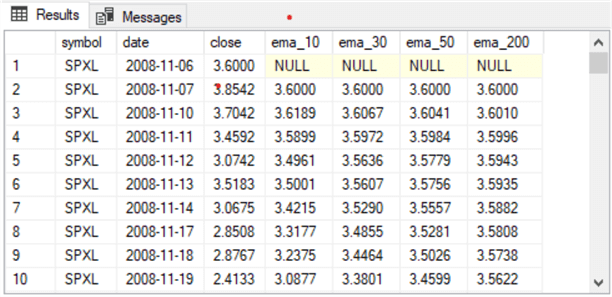
The table with the source data for each of the three tickers resides in a table named close_and_emas. The following pair of screenshots shows the first and last ten rows from this table.

• The first screenshot shows the first ten trading days for the SPXL ticker
  • The IPO date for this security is November 6, 2008
  • On the IPO date, the security closed at a value of 3.6000
  • There are four ema column values with column names of ema_10 for a period length of 10 trading days through ema_200 with a period length of 200 trading days.
    • The four ema column values for the initial public offering date all have null values. This is because the expression for an ema requires a close value for the preceding date, and there is no close value for the trading date before the IPO date
    • The ema column values for all the remaining trading dates depend on the close value for the current date and the ema value for the preceding trading date
• The second screenshot shows the last ten trading days for the UDOW ticker
  • The last row in the screenshot is for the last trading day for which values were collected and computed in the data for this tip. The date is November 30, 2022
  • All of these ten rows have close values as well as ema values
    • The close value is an observed value with one value for each trading date
    • The ema column values all have a preceding row with a close value because they display the final ten trading days for which data are available

The rows showing the trading day data for the TQQQ ticker are in the close_and_emas table from just after the last trading day for the SPXL ticker through just before the first trading day for the UDOW ticker. The rows within the close_and_emas table are ordered by ticker symbol in alphabetical order. The rows for each ticker symbol are ordered in ascending order by trading date. The following alter table statement shows the syntax for assigning a primary key constraint to the close_and_emas table that orders rows by trading date within ticker symbol. When there are no null values in any of the columns for a primary key, this constraint can remove the need for order by statements and consequently speed the performance of queries for the table.

alter table dbo.close_and_emas
add constraint symbol_date_pk PRIMARY KEY (symbol,date);

Overview of Contingency Tables, Row Categories, and Column Categories

All Chi Square homogeneity tests depend on at least two sets of categories. Each set of categories can be derived directly from a source data table or computed via a model and based on other content in a source data table. Both models examined in this tip depend either directly or indirectly on the close_and_emas table as their source data table.

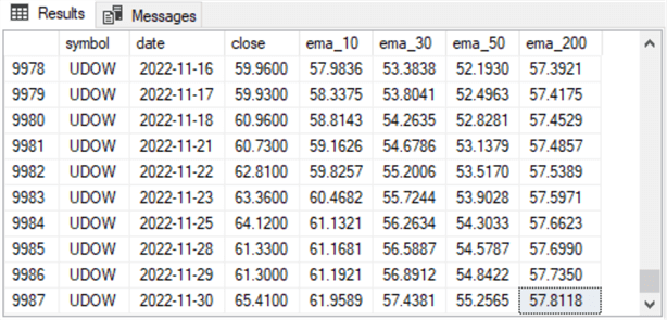
The two sets of categories are respectively for the rows and columns of a contingency table. The contingency table contains counts for the intersection of row categories with column categories from the source data table matching the row and column criteria for being in a cell of the contingency table. The following screen image shows a contingency table in a generalized format.

• The row categories are named Row 1, Row 2 through Row n
• Similarly, the column categories are named Column 1, Column 2 through Column n
• The cells within the body of the contingency table contain counts for the number of source data rows. The functions defining these cell counts can depend on data transformation expressions

As a SQL Server professional, your responsibilities will minimally include developing code to compute cell counts for the contingency table from the source data table. However, your contributions to a project can extend to assessing if the row counts across columns are homogeneous. The Chi Square homogeneity test offers a statistical basis for assessing if the distribution of counts across columns is homogeneous across rows in the contingency table.

This section illustrates the steps in a use case example of how to compute the cell counts for a contingency table based on a data model and a source data table. The model designates the criteria for rows from the source data table matching the classification criteria for cells in the contingency table.

In this first model for this tip, the categories are as follows.

• Row categories are for:
  • The close value for the current row being greater than the ema_10 value for the current row or
  • The close value for the current row not being greater than the ema_10 value
• Column categories are for ticker symbols. Recall that there are three ticker symbols (SPXL, TQQQ, and UDOW) tracked in the data for this tip. Each ticker is assigned to a column in the contingency table
• Therefore,
  • One set of classification identifiers within the contingency table is derived from a data model; these identifiers are for the rows of the contingency table
  • A second set of classification identifiers within the contingency table is derived from a column within the underlying SQL Server table for the contingency table
• The use case for this section illustrates another role for a data model besides designation of row or column identifiers for the contingency table. In this section, the data model also transforms three pairs of numeric column values into a metric to help evaluate the data underlying the contingency table

You can assess if the observed counts in the preceding generalized contingency table are proportional to all the contingency columns by comparing its observed counts to expected counts. The expressions for computing expected counts appear in the next screenshot. Notice that the expressions below depend on the row counts, the column counts, and the grand count.

To compare observed counts versus expected counts, represent observed counts by O_riciand expected counts by E_rici,.

• Let ri stand for the ith row category (Row 1, Row 2 through Row n)
• Let ci stand for the ith column category (Column 1, Column2, through Column n)

Then, compute a Chi Square component value for a single contingency table cell as (O_rici - E_rici)²/ E_rici. The Chi Square component value normalizes the magnitude of the squared difference between O_rici and E_ricito E_rici.

Next, sum the Chi Square component values for each cell in the contingency table. This sum is the Chi Square value for the counts in the observed counts table.

Finally, you can use a Chi Square probability value table to lookup or otherwise derive the probability of obtaining a Chi Square value greater than the computed Chi Square value. The entries along the top row in a Chi Square probability value table are the probabilities of obtaining a computed Chi Square as large or larger than the computed Chi Square value for a particular instance of a contingency table. A full explanation of how to apply Chi Square functions is way beyond the scope of this tip, but this tip does provide guidance and a specific example of how to apply the Chi Square test for homogeneity in its final subsection.

Towards a T-SQL Framework for Computing Custom Chi Square Homogeneity Tests

This section includes three subsections.

• The first subsection illustrates an approach to adding custom columns to the source data results set. The newly added columns are especially useful for specifying classification criteria for new contingency table classification sets based on an underlying source data table
• The second subsection presents T-SQL code for computing observed counts for a contingency table from an original or updated source data results set
• The third subsection presents T-SQL code for computing expected counts based on the observed counts computed in the second subsection. The third subsection also shows how to compute the Chi Square homogeneity statistic given the observed and expected counts for a contingency table. This subsection concludes with guidance on how to assess the homogeneity for the column values in the contingency table

Code for Adding New Columns to a Table of Operational Data in SQL Server

The next script excerpt adds four new column values to the operational data in the close_and_emas table.

• The first select statement begins with an asterisk that extracts all columns for the source data table in its from clause (close_and_emas)
  • The second, third, and fourth select list items depend on T-SQL lead functions. The lead function allows the display of data from subsequent rows to display on the same row as the current row. This feature is very useful when analyzing the relationship between current rows and future rows for time series data
    • The first lead function is for the close value that is five trading days beyond the current trading date. The name for this column of lead function values is close_lead_5
    • The second lead function is for the close value that is ten trading days beyond the current trading date. The name for this column of lead function values is close_lead_10
    • The third lead function is for the close value that is twenty trading days beyond the current trading date. The name for this column of lead function values is close_lead_20
  • The into clause copies the results set from the select statement to a new table named #close_and_emas_close_leads_5_10_20
• The second select statement builds on the #close_and_emas_close_leads_5_10_20 table by creating and populating a new table named #close_lead_5_close_lead_10_close_lead_20_gt_close via a select into statement. This statement additionally creates and populates some new columns
  • The close_gt_ema_10 column is required for the contingency table. The values in this column are 1 when the close value for the current row is greater than the ema_10 value; otherwise, the close_gt_ema_10 column value is 0 (even when one of the values being compared has a null value)
  • The close_lead_5_gt_close, close_lead_10_gt_close, and close_lead_20_gt_close columns are not required for the contingency table in this tip, but their discussion provides guidance about how to handle null values that you may find useful. The need for recognizing and correctly processing null values can easily arise for functions referencing preceding or trailing time series values. The code sample below shows a case statement syntax that assigns one of three values to a column when one of the values being compared is null
    • Null when one of two compared values is null
    • 1 when one of two compared values is greater than another non-null value
    • 0 when one of two compared values is not greater than another non-null value

use DataScience
go 
 
-- compute close_lead_5, close_lead_10_close_lead_20 column values
-- for joining to dbo.close_and_emas; saved joined results set to
-- #close_and_emas_close_leads_5_10_20
 
drop table if exists #close_and_emas_close_leads_5_10_20
 
select 
 *
,lead([close],5) over 
 (partition by symbol order by date) close_lead_5
,lead([close],10) over 
 (partition by symbol order by date) close_lead_10
,lead([close],20) over 
 (partition by symbol order by date) close_lead_20
 
into #close_and_emas_close_leads_5_10_20
from dbo.close_and_emas
 
-- optionally display with order by
-- select * from #close_and_emas_close_leads_5_10_20 order by symbol, date
 
-- compute close_gt_ema_10 column values along with 
-- close_lead_5_gt_close, close_lead_10_gt_close, and
-- close_lead_20_gt_close column values from 
-- #close_and_emas_close_leads_5_10_20; subset and save 
-- selected columns from the results set
-- to #close_lead_5_close_lead_10_close_lead_20_gt_close
 
drop table if exists #close_lead_5_close_lead_10_close_lead_20_gt_close
 
select 
-- originally from close_and_emas
 symbol
,date
,[close]
,ema_10
 
-- compute criterion values for each row
,
 case
  when [close] > ema_10 then 1
  else 0
 end close_gt_ema_10
 
-- compute criterion values for each column
-- close_lead_5_gt_close, close_lead_10_gt_close, 
-- close_lead_20_gt_close
,
 case
  when (close_lead_5 is not null) 
   and (close_lead_5 > [close]) then 1
  when (close_lead_5 is not null) 
   and (close_lead_5 <= [close]) then 0 
  else null
 end close_lead_5_gt_close
,
 case
  when (close_lead_10 is not null) 
   and (close_lead_10 > [close]) then 1
  when (close_lead_10 is not null) 
   and (close_lead_10 <= [close]) then 0 
   else null
 end close_lead_10_gt_close
,
 case
  when (close_lead_20 is not null) 
   and (close_lead_20 > [close]) then 1
  when (close_lead_20 is not null) 
   and (close_lead_20 <= [close]) then 0 
   else null
 end close_lead_20_gt_close
 
into #close_lead_5_close_lead_10_close_lead_20_gt_close
from #close_and_emas_close_leads_5_10_20
 
-- optionally display saved subset of results set columns
   select * 
   from #close_lead_5_close_lead_10_close_lead_20_gt_close
   order by symbol, date

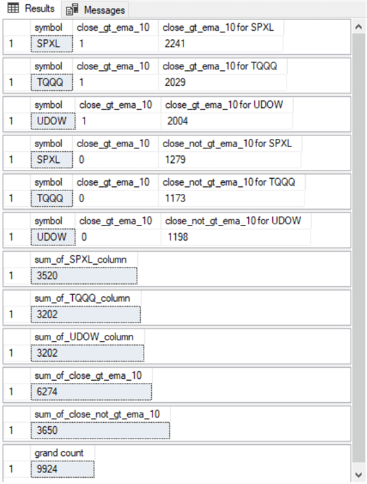
The next screenshot shows the first ten rows for the results set from the preceding script.

• All the rows are for the SPXL ticker starting with its IPO date of 2008-11-06.
• Therefore, the ema_10 column value is null on 2008-11-06
  • Consequently, the close_gt_ema_10 column value should be null, but it is instead 0. This is because the case statement for the column value does not include any special logic for handling null column values
  • This issue is resolved in the next subsection for this and other issues returning null values derived from the processing of the original source data results set
• The remaining nine rows in the screenshot have close_gt_ema_10 column values of 1 or 0 depending on whether the close value is greater than or not greater the ema_10 value

The next screenshot displays the last thirty rows for the results set from the preceding script.

• All the rows are for the UDOW ticker ending with the last day of data collection on November 30, 2022
• All the close_gt_ema_10 column values are 1 because each of the rows has a larger close value than its ema_10 value
• On the other hand, the close_lead_5_gt_close, close_lead_10_gt_close, and close_lead_20_gt_close columns end with 5, 10, or 20 rows of null values. Recall that these three columns unlike the close_gt_ema_10 column include special logic to handle comparison of two values when one of the values is null

Code for Computing Observed Contingency Cell, Column, Row, and Grand Counts

The next code excerpt shows the T-SQL for computing observed contingency cell, column, row, and grand counts. The query for computing each of these count values is derived from the #close_lead_5_close_lead_10_close_lead_20_gt_close table. Major sections within the script have a comment line describing the section's goal.

• For example, towards the top of the following script excerpt, there is a comment with text that reads: compute contingency cell counts
• The comments header for other major sections are
  • compute contingency column counts
  • compute contingency row counts
  • compute grand count

Within the query code for each set of counts, there is a where clause with special logic for filtering out null values for ema_10, close_lead_5_gt_close, close_lead_10_gt_close, and close_lead_20_gt_close columns. Consequently, the sum of the counts from these queries are less than the 9987 rows in the close_emas source data table. Instead, the sum of the counts for each set is 9924.

• For example, ema_10 values for a ticker's IPO date has a null value. This is because these dates have no preceding close value for the trading date before the IPO date
• Also, the close_lead_5_gt_close, close_lead_10_gt_close, and close_lead_20_gt_close columns end, respectively, with 5, 10, or 20 null values. These rows are for trading dates beyond the last date for which trading data was collected for this tip

There are six queries for the set of contingency cell counts.

• The from clause in each query references the #close_lead_5_close_lead_10_close_lead_20_gt_close table
• A group by clause in combination with select list items enable the computation of counts by symbol and close_gt_ema_10
• A pair of where clause criteria settings for close_gt_ema_10 and symbol column values designate the columns for which to extract counts; the order of the where clause criteria for the six select statements are
  • close_gt_ema_10 = 1 and symbol = 'SPXL'
  • close_gt_ema_10 = 1 and symbol = 'TQQQ'
  • close_gt_ema_10 = 1 and symbol = 'UDOW'
  • close_gt_ema_10 = 0 and symbol = 'SPXL'
  • close_gt_ema_10 = 0 and symbol = 'TQQQ'
  • close_gt_ema_10 = 0 and symbol = 'UDOW'

The next set of three queries compute contingency column counts -- one query per ticker symbol.

• The design of these three queries is very similar to the six queries for contingency cell counts.
• There is just one criterion setting for each symbol, and the order of the criterion settings are
  • symbol = 'SPXL'
  • symbol = 'TQQQ'
  • symbol = 'UDOW'

The next pair of queries has a comment header of contingency row counts.

• These queries are very similar to those for the contingency column counts, except there is just one query for each of two contingency table rows – one for each of two close_gt_ema_10 values
• There is just one criterion setting for each row count query. The order of the criterion settings are
  • close_gt_ema_10 = 1
  • close_gt_ema_10 = 0

There are at least three alternative approaches for computing the grand count. Recall that this count is for the count of all the rows from the #close_lead_5_close_lead_10_close_lead_20_gt_close table contributing rows to the grand count. The approach selected in this tip for computing the grand count is to assign each of the row counts to local variables named @close_gt_ema_10 and @close_not_gt_ema_10. These two local variables are set to adapted versions of the T-SQL for each of the two contingency row count queries.

• Each local variable is declared with an int data type.
• The grand count is just the sum of the two local variables added together inside the final select statement in the script below. The alias for the final select statement's result set is grand count.

use DataScience
go 
 
-- compute counts
 
-- compute contingency cell counts
select symbol, close_gt_ema_10, count_of_rows [close_gt_ema_10 for SPXL]
from
(
select symbol,close_gt_ema_10, count(*) count_of_rows
from #close_lead_5_close_lead_10_close_lead_20_gt_close 
where 
      ema_10 is not null and 
      close_lead_5_gt_close is not null and
      close_lead_10_gt_close is not null and
      close_lead_20_gt_close is not null
group by symbol,close_gt_ema_10
) for_row_displays
where 
   for_row_displays.close_gt_ema_10 = 1 and
   symbol = 'SPXL'
 
select symbol, close_gt_ema_10,count_of_rows [close_gt_ema_10 for TQQQ]
from
(
select symbol,close_gt_ema_10, count(*) count_of_rows
from #close_lead_5_close_lead_10_close_lead_20_gt_close 
where 
      ema_10 is not null and 
      close_lead_5_gt_close is not null and
      close_lead_10_gt_close is not null and
      close_lead_20_gt_close is not null
group by symbol,close_gt_ema_10
) for_row_displays
where 
   for_row_displays.close_gt_ema_10 = 1 and
   symbol = 'TQQQ'
 
select symbol, close_gt_ema_10,count_of_rows [close_gt_ema_10 for UDOW]
from
(
select symbol,close_gt_ema_10, count(*) count_of_rows
from #close_lead_5_close_lead_10_close_lead_20_gt_close 
where 
      ema_10 is not null and 
      close_lead_5_gt_close is not null and
      close_lead_10_gt_close is not null and
      close_lead_20_gt_close is not null
group by symbol,close_gt_ema_10
) for_row_displays
where 
   for_row_displays.close_gt_ema_10 = 1 and
   symbol = 'UDOW'
 
select symbol, close_gt_ema_10,count_of_rows [close_not_gt_ema_10 for SPXL]
from
(
select symbol,close_gt_ema_10, count(*) count_of_rows
from #close_lead_5_close_lead_10_close_lead_20_gt_close 
where 
      ema_10 is not null and 
      close_lead_5_gt_close is not null and
      close_lead_10_gt_close is not null and
      close_lead_20_gt_close is not null
group by symbol,close_gt_ema_10
) for_row_displays
where 
   for_row_displays.close_gt_ema_10 = 0 and
   symbol = 'SPXL'
 
select symbol, close_gt_ema_10,count_of_rows [close_gt_ema_10 for TQQQ]
from
(
select symbol,close_gt_ema_10, count(*) count_of_rows
from #close_lead_5_close_lead_10_close_lead_20_gt_close 
where 
      ema_10 is not null and 
      close_lead_5_gt_close is not null and
      close_lead_10_gt_close is not null and
      close_lead_20_gt_close is not null
group by symbol,close_gt_ema_10
) for_row_displays
where 
   for_row_displays.close_gt_ema_10 = 0 and
   symbol = 'TQQQ'
 
select symbol, close_gt_ema_10,count_of_rows [close_gt_ema_10 for UDOW]
from
(
select symbol,close_gt_ema_10, count(*) count_of_rows
from #close_lead_5_close_lead_10_close_lead_20_gt_close 
where 
      ema_10 is not null and 
      close_lead_5_gt_close is not null and
      close_lead_10_gt_close is not null and
      close_lead_20_gt_close is not null
group by symbol,close_gt_ema_10
) for_row_displays
where 
   for_row_displays.close_gt_ema_10 = 0 and
   symbol = 'UDOW'
 
 
-- compute contingency column counts
select sum(for_row_sums.count_of_rows) sum_of_SPXL_column
from
(
select symbol,close_gt_ema_10, count(*) count_of_rows
from #close_lead_5_close_lead_10_close_lead_20_gt_close 
where 
      ema_10 is not null and 
      close_lead_5_gt_close is not null and
      close_lead_10_gt_close is not null and
      close_lead_20_gt_close is not null
group by symbol,close_gt_ema_10
) for_row_sums
where symbol = 'SPXL'
 
select sum(for_row_sums.count_of_rows) sum_of_TQQQ_column
from
(
select symbol,close_gt_ema_10, count(*) count_of_rows
from #close_lead_5_close_lead_10_close_lead_20_gt_close 
where 
      ema_10 is not null and 
      close_lead_5_gt_close is not null and
      close_lead_10_gt_close is not null and
      close_lead_20_gt_close is not null
group by symbol,close_gt_ema_10
) for_row_sums
where symbol = 'TQQQ'
 
select sum(for_row_sums.count_of_rows) sum_of_UDOW_column
from
(
select symbol,close_gt_ema_10, count(*) count_of_rows
from #close_lead_5_close_lead_10_close_lead_20_gt_close 
where 
      ema_10 is not null and 
      close_lead_5_gt_close is not null and
      close_lead_10_gt_close is not null and
      close_lead_20_gt_close is not null
group by symbol,close_gt_ema_10
) for_row_sums
where symbol = 'UDOW'
 
 
-- compute contingency row counts
select sum(for_row_sums.count_of_rows) sum_of_close_gt_ema_10
from
(
select symbol,close_gt_ema_10, count(*) count_of_rows
from #close_lead_5_close_lead_10_close_lead_20_gt_close 
where 
      ema_10 is not null and 
      close_lead_5_gt_close is not null and
      close_lead_10_gt_close is not null and
      close_lead_20_gt_close is not null
group by symbol,close_gt_ema_10
) for_row_sums
where close_gt_ema_10 = 1
 
select sum(for_row_sums.count_of_rows) sum_of_close_not_gt_ema_10
from
(
select symbol,close_gt_ema_10, count(*) count_of_rows
from #close_lead_5_close_lead_10_close_lead_20_gt_close 
where 
      ema_10 is not null and 
      close_lead_5_gt_close is not null and
      close_lead_10_gt_close is not null and
      close_lead_20_gt_close is not null
group by symbol,close_gt_ema_10
) for_row_sums
where close_gt_ema_10 = 0
 
 
-- compute grand count
declare @close_gt_ema_10 int =
(
-- compute contingency row counts
select sum(for_row_sums.count_of_rows) sum_of_close_gt_ema_10
from
(
select symbol,close_gt_ema_10, count(*) count_of_rows
from #close_lead_5_close_lead_10_close_lead_20_gt_close 
where 
      ema_10 is not null and 
      close_lead_5_gt_close is not null and
      close_lead_10_gt_close is not null and
      close_lead_20_gt_close is not null
group by symbol,close_gt_ema_10
) for_row_sums
where close_gt_ema_10 = 1
)
 
 
declare @close_not_gt_ema_10 int =
(
select sum(for_row_sums.count_of_rows) sum_of_close_not_gt_ema_10
from
(
select symbol,close_gt_ema_10, count(*) count_of_rows
from #close_lead_5_close_lead_10_close_lead_20_gt_close 
where 
      ema_10 is not null and 
      close_lead_5_gt_close is not null and
      close_lead_10_gt_close is not null and
      close_lead_20_gt_close is not null
group by symbol,close_gt_ema_10
) for_row_sums
where close_gt_ema_10 = 0
)
 
select (@close_gt_ema_10 + @close_not_gt_ema_10) [grand count]

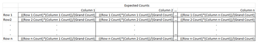
The following screenshot shows the results sets generated by the preceding script excerpt. There are twelve results sets returned by the script excerpt. Because each of the twelve queries in the script reference the #close_lead_5_close_lead_10_close_lead_20_gt_close table in its from clause, all results are for source data from that table. The values in these results sets are important for computing expected counts and Chi Square statistics for evaluating the homogeneity of the cell counts in a contingency table.

• The first six results sets are returned by the queries from the compute contingency cell counts section from the preceding script
  • The first three of these results sets are for the SPXL, TQQQ, and UDOW ticker symbols for rows that have a greater close value than their ema_10 value
  • The second three results sets are for rows for the SPXL, TQQQ, and UDOW ticker symbols for rows that do not have a greater close value than their ema_10 value
• The seventh through the ninth results sets are returned from the compute contingency column counts section in the preceding script
  • The seventh results set is for counts from cells for ticker symbols with a SPXL value
  • The eighth results set is for counts from cells for ticker symbols with a TQQQ ticker
  • The ninth results set is for counts from cells for ticker values of UDOW
• The tenth and eleventh results sets are returned from the compute contingency row counts section of the preceding script
  • The tenth results set is for the count of rows that have a close_gt_ema_10 column value of 1. The value for this results set (6274) is the number of rows for which the close value is greater than the ema_10 value
  • The eleventh results set is for counts that have a close_gt_ema_10 column value of 0. The value for this results set (3650) is the number of rows for which the close value is greater than the ema_10 value
  • Notice that the sum of 6274 and 3650 is 9924, which is the number or rows with non-null values for ema_10, close_lead_5_gt_close, close_lead_10_gt_close, close_lead_20_gt_close in the #close_lead_5_close_lead_10_close_lead_20_gt_close table
• The twelfth results set is returned from the compute grand count section of the preceding script. The grand count results set returns a value of 9924
  • As indicated in the discussion of the tenth and eleventh results sets, this results set's return value is the sum of the row counts for cells with close value greater their ema_10 value as well as for cells with a close value not greater than their ema_10 value
  • You can get to the same return value by summing the column counts in the seventh through the ninth results sets or by summing the cell counts in the first through the sixth results sets

Code for Computing Expected Counts and the Chi Square Test Value for Homogeneity

The final T-SQL script excerpt in this tip implements the steps remaining after the observed counts are computed through to the computation of the Chi Square statistic for homogeneity along with its corresponding degrees of freedom. These steps are as follows:

• Compute expected cell counts for the contingency table
• Compute the Chi Square component for each cell in the contingency table
• Sum the Chi Square component values across contingency table cells
• Compute the degrees of freedom for the computed Chi Square statistic
• Evaluate the computed Chi Square statistic as indicating or not indicating homogeneity

The following script starts by re-listing with a set of six select statements the observed cell counts computed towards the end of script in the preceding subsection. For ease of presentation and re-using results set values, the six select statements commence by displaying a scalar constant with an appropriate alias value for each observed cell count.

After displaying the observed cell count values computed in the script for the preceding subsection, the following script implements the expressions for the expected cell counts from the "Overview of contingency tables, row categories, and column categories" section. For example, the expected count for the expected close_gt_ema_10 for the SPXL cell depends on three values

• A Row 1 Count value of 6274
• A Column 1 Count value of 3520
• A grand count value of 9924

Expected counts are computed and displayed via select statements for the remaining five cells in the contingency table based on column counts, row counts, and the grand count.

Next, the code computes Chi Square components for each of the six cells in the contingency table one row at time. The Chi Square components are based on the squared difference between observed and expected cell counts normalized by the expected count for a cell.

• The three column values for the first row are
  • For each of the three ticker symbols tracked in the tip
  • For the row of component values in which current row close values are greater than corresponding ema_10 column values for the current row in the underlying data source
• The three column values for the second row are
  • For each of the three ticker symbols tracked in this tip
  • For the row of component values in which the current row close values are not greater than corresponding ema_10 column values for the current row in the underlying data source
• A local variable is named and defined via a T-SQL expression for each of the three columns for a row of tickers
  • The local variable names for the row with close values greater than ema_10 values are
    • @close_gt_ema_10_for_SPXL_diff
    • @close_gt_ema_10_for_TQQQ_diff
    • @close_gt_ema_10_for_UDOW_diff
  • The local variable names for the row with close values not greater than ema_10 values are
    • @close_nt_gt_ema_10_for_SPXL_diff
    • @close_nt_gt_ema_10_for_TQQQ_diff
    • @close_nt_gt_ema_10_for_UDOW_diff
• After completing the computations for the squared differences between observed and expected counts along with the corresponding component values for the column values on a row, the code concatenates squared differences and component values with union operators
• The Chi Square statistic is computed as the sum of the Chi Square components across contingency table cells
• The statistical assessment of homogeneity depends on three factors
  • In general, the larger the Chi Square test statistic, the less homogeneous cell counts are across contingency table columns
  • The statistical assessment for homogeneity also depends on the value of the degrees of freedom for the contingency table
    • The degrees of freedom for the contingency table for the example in this tip is 2
    • In general, you can compute the degrees of freedom for a contingency table as number of columns less 1 times the number of rows less 1
  • The critical Chi Square value at a specified probability level of significance
    • Technical analysts normally use a critical probability level of significance of 5%
    • If your requirements warrant, you can create, populate, and reference a table of critical Chi Square values with degrees of freedom and probability levels; here is an online reference to a table of critical Chi Square values
    • Then, your code can compare the looked-up value from the table to the computed Chi Square value for the contingency table being analyzed for homogeneity
  • If the computed Chi Square test statistic is greater than or equal to the critical Chi Square value, then the assumption of homogeneity is rejected
  • The script below uses default assignments for the degrees of freedom, the critical Chi Square value for homogeneity, and implicitly a significance probability level (namely, 5%)
• A previously published MSSQLTips.com article demonstrates how to populate programmatically with T-SQL a table of critical Chi Square values at different statistical significance levels as well as how to compare a computed Chi Square statistic to a critical Chi Square value

-- compute and display observed and expected cell 
-- row, column, and grand counts
 
-- observed cell count values
select (2241) [close_gt_ema_10 for SPXL]
select (2029) [close_gt_ema_10 for TQQQ]
select (2004) [close_gt_ema_10 for UDOW]
select (1279) [close_not_gt_ema_10 for SPXL]
select (1173) [close_not_gt_ema_10 for TQQQ]
select (1198) [close_not_gt_ema_10 for UDOW]
 
-- computed expected count values
select ((6274 * 3520)/9924) [expected close_gt_ema_10 for SPXL]
select ((6274 * 3202)/9924) [expected close_gt_ema_10 for TQQQ]
select ((6274 * 3202)/9924) [expected close_gt_ema_10 for UDOW]
select ((3650 * 3520)/9924) [expected close_not_gt_ema_10 for SPXL]
select ((3650 * 3202)/9924) [expected close_not_gt_ema_10 for TQQQ]
select ((3650 * 3202)/9924) [expected close_not_gt_ema_10 for UDOW]
 
-----------------------------------------------------------------------
 
-- compute and display squared differences and components
-- between observed and expected cell counts
-- across contingency cells based on
-- close values gt ema_10 values
 
declare @close_gt_ema_10_for_SPXL_diff int 
 = 
 power(
  (
   select (2241) 
   - 
   (select ((6274 * 3520)/9924))
  )
 ,2)
 
,@close_gt_ema_10_for_TQQQ_diff int 
 = 
 power(
  (
   select (2029) 
   - 
   (select ((6274 * 3202)/9924))
  )
 ,2)
 
,@close_gt_ema_10_for_UDOW_diff int 
 = 
 power(
  (
   select (2004) 
   - 
   (select ((6274 * 3202)/9924))
  )
 ,2)
 
 
 -- display squared differences and components
select 
 2241 [observed]
,(select ((6274 * 3520)/9924)) [expected]
,@close_gt_ema_10_for_SPXL_diff [squared difference of O and E]
,cast(@close_gt_ema_10_for_SPXL_diff as float)
 /
 cast((select ((6274 * 3520)/9924)) as float) [component]
 
union
 
select
 2029 [observed]
,(select ((6274 * 3202)/9924)) [expected]
,@close_gt_ema_10_for_TQQQ_diff [squared difference of O and E]
,cast(@close_gt_ema_10_for_TQQQ_diff as float)
 /
 cast((select ((6274 * 3202)/9924)) as float) [component]
 
union
 
select
 2004 [observed]
,(select ((6274 * 3202)/9924)) [expected]
,@close_gt_ema_10_for_UDOW_diff [squared difference of O and E]
,cast(@close_gt_ema_10_for_UDOW_diff as float)/ cast((select ((6274 * 3202)/9924)) as float) [component]
 
 
 
-- compute and display squared differences and components
-- between observed and expected cell counts
-- across contingency cells based on
-- close values not gt ema_10 values
 
declare @close_not_gt_ema_10_for_SPXL_diff int 
 = 
 power(
  (
   select (1279) 
   - 
   (select ((3650 * 3520)/9924))
  )
 ,2)
 
,@close_not_gt_ema_10_for_TQQQ_diff int 
 = 
 power(
  (
   select (1173) 
   - 
   (select ((3650 * 3202)/9924))
  )
 ,2)
 
,@close_not_gt_ema_10_for_UDOW_diff int 
 = 
 power(
  (
   select (1198) 
   - 
   (select ((3650 * 3202)/9924))
  )
 ,2)
 
 -- display squared differences and components
select 
 1279 [observed]
,(select ((3650 * 3520)/9924)) [expected]
,@close_not_gt_ema_10_for_SPXL_diff [squared difference of O and E]
,cast(@close_not_gt_ema_10_for_SPXL_diff as float)/ cast((select ((3650 * 3520)/9924)) as float) [component]
 
union
 
select
 1173 [observed]
,(select ((3650 * 3202)/9924)) [expected]
,@close_not_gt_ema_10_for_TQQQ_diff [suared difference of O and E]
,cast(@close_not_gt_ema_10_for_TQQQ_diff as dec(19,0))/ cast((select ((3650 * 3202)/9924)) as dec(19,0)) [component]
 
union
 
select
 1198 [observed]
,(select ((3650 * 3202)/9924)) [expected]
,@close_not_gt_ema_10_for_UDOW_diff [squared difference of O and E]
,cast(@close_not_gt_ema_10_for_UDOW_diff as float)/ cast((select ((3650 * 3202)/9924)) as dec(19,0)) [component]
 
-----------------------------------------------------------------------
 
-- compute aggregated component values for contingency cells
select sum(cast([component value] as float)) [Chi Square test statistic]
from
(
select
 '@close_gt_ema_10_for_SPXL_diff' [component identifier]
,cast(@close_gt_ema_10_for_SPXL_diff as float)
 /
 cast((select ((6274 * 3520)/9924)) as float) [component value]
 
 union
 
 select
 '@close_gt_ema_10_for_TQQQ_diff' [component identifier]
,cast(@close_gt_ema_10_for_TQQQ_diff as float)
 /
 cast((select ((6274 * 3202)/9924)) as float)
 
 
 union
 
 select
 '@close_gt_ema_10_for_UDOW_diff' [component identifier]
,cast(@close_gt_ema_10_for_UDOW_diff as float)
 /
 cast((select ((6274 * 3202)/9924)) as float)
 
 
 union
 
select
 '@close_not__gt_ema_10_for_SPXL_diff' [component identifier]
,cast(@close_not_gt_ema_10_for_SPXL_diff as float)
 /
 cast((select ((3650 * 3520)/9924)) as float) [component value]
 
 
 union
 
select
 '@close_not__gt_ema_10_for_TQQQ_diff' [component identifier]
,cast(@close_not_gt_ema_10_for_TQQQ_diff as float)
 /
 cast((select ((3650 * 3202)/9924)) as float) [component value]
 
 
 union
 
select
 '@close_not__gt_ema_10_for_UDOW_diff' [component identifier]
,cast(@close_not_gt_ema_10_for_UDOW_diff as float)
 /
 cast((select ((3650 * 3202)/9924)) as float) [component value]
) for_component_identifiers_and_values
 
-- degrees of freedom calculator for a contingency table 
-- with a default setting of 2 rows and 3 columns
declare @rows int = 2, @columns int = 3
select ((@rows-1)*(@columns-1)) [degrees of freedom]
 
-- assign critical Chi Square value at 5% probability here
-- and assign default @Chi_Square_test_statistic = .887
declare 
 @Critical_Chi_Square_at_5_percent float = 5.991
,@Chi_Square_test_statistic float= .887
-- report homogeneity 3650 outcome
if @Chi_Square_test_statistic >= @Critical_Chi_Square_at_5_percent
   begin
      select 'The cell counts are not homogeneous'
   end
else
   begin
      select 'The cell counts are homogeneous'
   end 

There are two main parts to the output from the preceding script.

The first part consists of twelve results sets with actual and expected counts for the contingency table cells. The first 6 of the 12 rows show observed cell counts originally computed and reported in the preceding subsection. The second 6 of the 12 rows show the computed expected counts for the contingency table. Here is a display with these 12 rows.

Here is the output from the second part of the preceding script.

• The output begins with two sets of three rows. One row in each set of three rows is for a ticker symbol, namely SPXL, TQQQ, and UDOW
  • The first set of three rows is for comparisons based on when the close value is greater than the ema_10 value in the underlying data source for the contingency table
  • The second set of three rows is for comparisons based on when the close value is not greater than the ema_10 value in the underlying data source for the contingency table
• The last column in the first and second set of three rows is for the computed Chi Square component value for a cell in the contingency table. The sum of these Chi Square component values is the Chi Square test statistic value (0.887191136640955) for the contingency table
• The next to the last pane in the output below is the computed degrees of freedom for the contingency table (2).
• The output that appears in the final pane of the screenshot below is generated by an IF…ELSE statement
  • When the computed Chi Square test statistic is greater than or equal to the Chi Square critical value, the IF…ELSE statement indicates the contingency table does not contain homogeneous column values
  • When the computed Chi Square statistic is not greater than or equal to the critical Chi Square value, the IF…ELSE statement indicates the hypothesis of homogeneous column values for the contingency table cannot be rejected (this is an alternative way of saying homogeneity across column values is accepted)
  • Because the computed Chi Square statistic in the example for this tip is not greater than or equal to the Chi Square critical value, the output reports that the cell counts are homogeneous

Next Steps

The very next step after reading this tip is to decide if you want a hands-on experience with the techniques demonstrated in it. You can get the code you need for a hands-on experience from the code windows in the tip. However, if you want to run the code exactly as it is described in the tip, then you also need the clos_and_emas table. The tip's download includes a csv file with the data for the table. After loading the csv file contents into a SQL Server, the code should run exactly as described in the tip.

Another next step is to experiment applying the techniques discussed in the article to a table with fresh data. This tip includes a link to Yahoo Finance for downloading data to a csv file. Please be aware that Yahoo Finance downloads csv files in a UNIX instead of a Microsoft file format. SQL Server, especially earlier versions, do not read UNIX files. One work-around to this formatting issue involves importing a UNIX-style csv file into Excel, which automatically recognizes UNIX-style csv files. Then, save the file from Excel as a Microsoft csv file.

Yet another next step is to apply the techniques from this article to a copy of any production-level table to which you have access. The table copy should have a primary key for each row. Additionally, the table should have some columns with classification identifiers, such as for the rows and columns of a contingency table. If necessary, you can add new columns to your copy of a production-level table. You can get ideas on how to add new columns with row and column identifiers from the subsection titled "Code for adding new columns to a table of operational data in SQL Server". This table will serve as your underlying data source for the Chi Square homogeneity test.

About the author

Rick Dobson is an author and an individual trader. He is also a SQL Server professional with decades of T-SQL experience that includes authoring books, running a national seminar practice, working for businesses on finance and healthcare development projects, and serving as a regular contributor to MSSQLTips.com. He has been growing his Python skills for more than the past half decade -- especially for data visualization and ETL tasks with JSON and CSV files. His most recent professional passions include financial time series data and analyses, AI models, and statistics. He believes the proper application of these skills can help traders and investors to make more profitable decisions.

This author pledges the content of this article is based on professional experience and not AI generated.

View all my tips