By: Rick Dobson | Comments | Related: > TSQL
Problem
Users with time series data on database servers often want to learn how to compute moving averages for time series data. Please introduce this topic for database administrators by focusing on the differences between simple moving averages (SMA) versus exponential moving averages (EMA).
Solution
Time series data consists of measurements or observations over a sequence of periods. The measurements can be for the rain at a weather station, the close price of a stock at a stock market, or the hospitalizations with a primary diagnosis of corona virus in a state. Time series periods can correspond to day parts, days, weeks, months, quarters, years, etc.
Time series data often have trends across a set of time periods. However, discernment of these trends can be obscured by random variations from one period to the next. Moving averages can help to highlight the direction of a trend if there is one. Some typical questions about trends that moving averages can help to answer include:
- Are sales decreasing or increasing in the short-term?
- Are stock prices beginning to reverse direction from rising to falling or vice versa?
- Are hospitalizations declining for corona virus?
Two especially common moving averages are simple moving averages and exponential moving averages. Both kinds of moving averages report one smoothed time series value per period. Simple moving averages can be thought of as a kind of partitioned database approach to smoothing time series data. In contrast, an exponential moving average takes a non-partitioned database approach to smoothing time series data.
Logic for computing simple moving averages
Simple moving averages smooth a time series by computing a succession of arithmetic averages over a sequence of periods. The beginning and ending periods for each moving average changes by one period from the first simple moving average through the last simple moving average for a time series.
- When computing a ten-period simple moving average, the average of the first ten points is assigned to the tenth period in the time series.
- Ten-period moving averages corresponding to the first nine periods of a ten-period moving average have a null value. These nine periods have null values because the expression for a ten-period simple moving average does not compute until after the ninth period.
- The second ten-period simple moving average is the average of the second through the eleventh time series values.
- Each successive ten-period moving average is the average of another progressive set of ten time series values.
You can think of a simple moving average as a partitioned database approach to smoothing time series data. The following process description is for a set of ten-period simple moving averages.
- The first ten-period simple moving average is based on the first ten periods or partitions. A partition consists of a single time series value in a period.
- The second simple moving average is based on the second through the eleventh partitions. This definition drops the first period from the first simple moving average and adds the eleventh period.
- The last ten-period simple moving average for a set of time series values is derived from the last time series value and the preceding nine time series values.
The arithmetic moving average for each set of periods are a smoothed version of the underlying time series values. An arithmetic average is computed as the sum of a set of values divided by the number of values in the period length for a simple moving average. Therefore, each underlying value has a weight that is one divided by the number of periods for the simple moving average.
A time series can have multiple moving averages where each moving average has a different period length. The period length generally corresponds to the size of a window in a T-SQL windows function, such as the windows avg() function. Common moving average period lengths for stock prices are ten-period and twenty-period moving averages. There are slightly more than twenty trading days per month. A ten-period moving average reflects the prices in about a half of a month.
Logic for computing exponential moving averages
Exponential moving averages depend on the weighted average of two values per period.
- The first value is the underlying time series value for the current period.
- The second value, with one exception, is the exponential moving average for the prior period.
- The weights for the weighted average are
- alpha for the first value and
- 1 – alpha for the second value
- so that alpha is typically greater than 0 and less than 1
Because of these specifications, it is impossible to compute an exponential moving average for the first period in a time series. This is because there can be no prior exponential moving average for the first period in a time series.
Also, the exponential moving average for the second underlying value depends on an arbitrary assignment of the prior exponential moving average.
- One common assumption is to use the first time series value as the exponential moving average for the prior period when computing the exponential moving average for the second time series value.
- Another common approach is to use the arithmetic average of the first four or five underlying time series values.
The value of alpha can depend on the profession in which the exponential moving average is being used.
- In financial applications, the value of alpha is typically 2 divided by
the period length value plus one for the exponential moving average. Therefore,
the values of alpha are
- 2/11 for a ten-period exponential moving average
- 2/21 for a twenty-period exponential moving average
- 2/31 for a thirty-period exponential moving average
- In engineering and mathematical applications, it is common to search for a value of alpha that minimizes the sum of squared differences between the exponentially smoothed average values and the underlying time series values. When you use this approach, then there is no notion of multiple exponential moving averages for an underlying time series. There is just the exponentially smoothed values that correspond to the closest fit of the smoothed values to the underlying time series values.
There are a couple of conceptual differences beyond those mentioned above in how to compute exponential moving averages versus simple moving averages for an underlying set of time series values.
- Simple moving averages are computed for a window that encompasses a set of underlying time series values. This window is the period length of the simple moving average. Therefore, as earlier values fail to fall within the computational window, they are discarded. In contrast, exponential moving averages go back consistently to the second underlying time series value -- no matter what the period length is for an exponential moving average and no matter how many underlying values exist in the time series.
- Simple moving averages are always null for the first period length minus one underlying time series values. This means that a ten-period simple moving average series starts with nine null values. By extension, a two-hundred-period simple moving average starts with one-hundred-ninety-nine null values. In contrast, an exponential moving average series always starts with just one null value, which is for the first underlying time series value.
A T-SQL example for computing simple moving averages
This section illustrates the basics of how to compute simple moving averages with T-SQL in SQL Server. Before starting the demonstration of how to compute simple moving averages, this section begins with a demonstration of reading some time series values into a SQL Server table.
Reading time series values into to a SQL Server table
This initial programming step in the tip relies on a .csv file with time series values. These data are for stock close prices for the QQQ symbol. This symbol is for an index based on the leading 100 or so stocks traded on the NASDAQ stock exchange. The periods are for trading days starting on January 4, 2021 through May 14, 2021. The data are typical open-high-low-close-volume data.
Here is the T-SQL script for importing the .csv file with time series data into a SQL Server table.
- The script starts with a reference to the DataScience database. You can change the name to any other database you prefer to use.
- A drop table if exists statement removes any previously existing version of the qqq_jan_may_2021 table in the dbo schema of the default database (DataScience).
- Next, a create table statement specifies the columns for the qqq_jan_may_2021 table.
- Then, a bulk insert statement is invoked to copy the values from the QQQ_Jan_May_2021.csv file to the qqq_jan_may_2021 table. The bulk insert operation starts from the second row in the .csv file (firstrow = 2) because the first row contains column headers. Make sure the .csv file resides in a location to which the SQL Server instance has access.
- Finally, a select statement displays the imported contents from the .csv file.
-- reference a database
use DataScience
go

--conditionally create a table
drop table if exists dbo.qqq_jan_may_2021;

create table dbo.qqq_jan_may_2021(
date date,
[open] money,
[high] money,
[low] money,
[close] money,
[volume] bigint
)

-- bulk insert with SQL Server
bulk insert dbo.qqq_jan_may_2021
from 'c:\DataScienceSamples\QQQ_Jan_May_2021.csv'
with(format='csv',firstrow = 2);

-- display imported csv file
select * from dbo.qqq_jan_may_2021
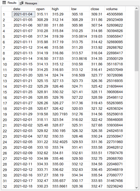
The following screen shot shows the contents of the first thirty-two rows in the qqq_jan_may_2021 table in the Results tab of a SSMS window.
- The data has six columns named: date, open, high, low, close and volume.
- This tip only requires two columns:
- The date column is for specifying periods in the time series within the qqq_jan_may_2021 table.
- The close column is for specifying the underlying time series values. The close column represents the closing price for the QQQ index on a trading date denoted by the date column value.
Computing simple moving averages with period lengths of ten, twenty, and thirty
Here is a script for computing simple moving averages with three period lengths for the time series from January 4, 2021 through May 14, 2021.
- The script starts with a drop table if exists statement for the close_sma_10_sma_20_sma_30 table.
- Next, a select statement with an into clause computes ten, twenty, and thirty
period simple moving averages.
- Each of the three moving averages are computed with a case statement inside the select statement. The column names for the case statements are, respectively, sma_10, sma_20, and sma_30.
- The when clause within each case statement computes the simple moving averages after enough close prices are collected to start computing non-null simple moving averages.
- The else clause within each case statement assigns a null value when there are insufficient values at the beginning of the time series to compute a simple moving average.
- The final select statement displays the contents of the close_sma_10_sma_20_sma_30 table.
-- create a fresh copy of dbo.close_sma_10_sma_20_sma_30
drop table if exists dbo.close_sma_10_sma_20_sma_30;

-- compute 10, 20, and 30 period sma's
select
 date date
,[close] [close]
-- for ten-period moving average
,
case
   when row_number() OVER(ORDER BY [Date]) > 9
      then avg([Close]) OVER(ORDER BY [Date] ROWS BETWEEN 9 PRECEDING AND CURRENT ROW)
   else null
end sma_10
-- for twenty-period moving average
,
case
   when row_number() over(order by [date]) > 19
      then avg([close]) over(order by [date] rows between 19 preceding and current row)
   else null
end sma_20
-- for thirty-period moving average
,
case
   when row_number() over(order by [date]) > 29
      then avg([close]) over(order by [date] rows between 29 preceding and current row)
   else null
end sma_30
into dbo.close_sma_10_sma_20_sma_30
from dbo.qqq_jan_may_2021

select * from dbo.close_sma_10_sma_20_sma_30
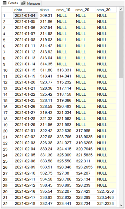
Here are the first thirty-two rows from the close_sma_10_sma_20_sma_30 table. The full set of rows in the table extend through May 14, 2021.
- There is a separate row for each trading date.
- For example, the first five rows are for trading dates from 2021-01-04 through 2021-01-08. These are the first five trading dates in 2021.
- There is no row for 2021-01-18, which is a holiday on which the US stock markets are closed. There are also no rows for dates falling on Saturdays and Sundays when the US stock markets are also closed.
- Each row has five column values for date, close, sma_10, sma_20, and sma_30.
- The first nine rows of the sma_10 column contain NULL values. All remaining rows in this column contain a ten-period simple moving average for the ten trading days ending on the date row value.
- The first nineteen rows of the sma_20 column and the first 29 rows of the sma_30 columns also display, respectively, NULL values. Otherwise, these two columns contain, respectively, twenty-period and thirty-period simple moving averages.
A T-SQL example for computing exponential moving averages
The computational example for the exponential moving average sample in this section of the tip uses the same time series source data as in the preceding section. If you have not already populated the source data table (dbo.qqq_jan_may_2021), then run the code from the preceding section to accomplish that goal before running the example code in this section.
After the source data becomes available in the dbo.qqq_jan_may_2021 table, the example in this section commences by creating a destination table (dbo.qqq_jan_may_2021_with_ema_cols) for storing the exponential moving averages. As with the simple moving average computational example, this section demonstrates the computation of moving averages with three different period lengths (ema_10 for ten-period exponential moving averages, ema_20 for twenty-period exponential moving averages, and ema_30 for thirty-period moving averages). The destination table contains three sets of columns:
- Two identifier columns for the sequential rows in the table.
- Row_number with a sequence of row numbers in the order of the dates for the source time series data.
- Date with a sequence of date values derived from the source time series data.
- The third column contains just the close column values from the source data table. The open, high, low, and volume columns from the source data table are not required for the example in this section (or, for that matter, in the preceding section on simple moving averages).
- The last three columns are for the three moving averages with different period lengths (ema_10, ema_20, and ema_30).
Here is a T-SQL script for creating the dbo.qqq_jan_may_2021_with_ema_cols destination table. The example code populates the first two sets of columns, but it leaves the last three columns for exponential moving averages with null values. The code for populating the ema_10, ema_20, and ema_30 columns depends on values in the row_number and close columns. Therefore, these two columns are populated prior to populating the ema_10, ema_20, and ema_30 columns.
- The drop table if exists and create table statements create a fresh copy of the dbo.qqq_jan_may_2021_with_ema_cols destination table.
- The insert…select statement populates the first two sets of columns
in the destination table.
- The row_number column values are populated via a T-SQL windows row_number() function in the select statement. The order by clause in the function specifies that row number values progress from the first through the last date in the source time series table (dbo.qqq_jan_may_2021).
- The date and close column values are derived from the date and close columns of the source time series table.
- The final select statement in the script displays the partially populated dbo.qqq_jan_may_2021_with_ema_cols destination table.
-- conditionally create table for close and emas
drop table if exists dbo.qqq_jan_may_2021_with_ema_cols;

create table dbo.qqq_jan_may_2021_with_ema_cols(
row_number bigint,
date date,
[close] money,
ema_10 money,
ema_20 money,
ema_30 money
)

insert dbo.qqq_jan_may_2021_with_ema_cols
(
row_number,
date,
[close]
)
select row_number() over(order by date) row_number, date, [close] from dbo.qqq_jan_may_2021

select * from dbo.qqq_jan_may_2021_with_ema_cols
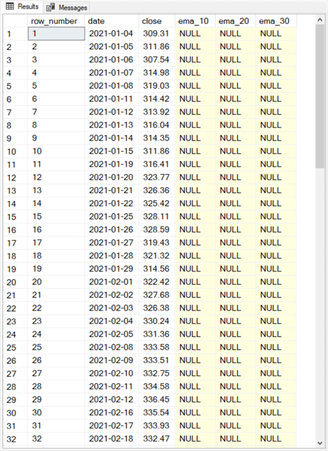
The following screen shot shows the first thirty-two rows from the select statement at the bottom of the preceding script. For this excerpt from the results set
- The row_number values progress from 1 through 32.
- The date values start at 2021-01-04 and advance for each subsequent trading date.
- The close values match the source time series values for the simple moving average example.
- The ema_10, ema_20, and ema_30 column values are all null. These values are populated in the next code segment.
Here is the code for populating the ema_10, ema_20, and ema_30 column values in the dbo.qqq_jan_may_2021_with_ema_cols table. It is designed to run immediately after the preceding code segment.
- The declarations at the top of the script are for the alpha weights. The
ten-period, twenty-period, and thirty-period exponential moving averages each
have their own alpha weight.
- @ema_10_alpha is for computing the ten-period moving average values
- @ema_20_alpha is for computing the twenty-period moving average values
- @ema_30_alpha is for computing the thirty-period moving average values
- A comment line immediately after the declarations reminds you that there is no exponential moving value for the first time series value.
- The update statement after the comment line assigns the close value from the first row as the exponential moving average for the second row of the table.
- Next, a declare statement assigns some values for looping through the third
through the last row of the table.
- The @count_of_rows local variable has a value that matches the row_number value for the last row in the table.
- The @current_rownumber local variable has a value that points at the current row number in the loop through the table’s rows. This local variable is initialized to 3.
- The @prior_rownumber local variable has a value that points at the row before the current row in the loop. This local variable is initialized to 2.
- Next, a while statement initializes the loop so that it starts at the beginning
value of @current_rownumber (3).
- The code inside the loop increments @current_rownumber by 1 for each pass through the loop.
- The code inside the loop also increments @prior_rownumber by 1 for each pass through the loop.
- The loop ends when @current_rownumber increments to a value greater than @count_of_rows.
- A begin…end code block after the while statement marks the beginning and end of the loop.
- An update statement with a set statement computes the exponentially weighted smoothed time series value for each period length. This set statement assigns values to the ema_10, ema_20, and ema_30 columns within the table.
- The select statement at the end of the following script segment displays the fully populated dbo.qqq_jan_may_2021_with_ema_cols table.
-- declarations for ema weights
declare
 @ema_10_alpha float =(2.0/11.0)
,@ema_20_alpha float =(2.0/21.0)
,@ema_30_alpha float =(2.0/31.0)

-- there are no ema's on row_number 1 by definition

-- assign values to ema's on row_number 2
-- simple definition is to use close from row_number 1
update dbo.qqq_jan_may_2021_with_ema_cols
set ema_10 =(select [close] from dbo.qqq_jan_may_2021_with_ema_cols where row_number = 1),
    ema_20 =(select [close] from dbo.qqq_jan_may_2021_with_ema_cols where row_number = 1),
    ema_30 =(select [close] from dbo.qqq_jan_may_2021_with_ema_cols where row_number = 1)
where row_number = 2;

declare
 @current_rownumber bigint = 3
,@prior_rownumber bigint = 2
,@count_of_rows bigint =
   (select count(*) from dbo.qqq_jan_may_2021_with_ema_cols)

while @current_rownumber <= @count_of_rows
begin

--select @prior_rownumber, @current_rownumber, @count_of_rows
-- assign values to ema's on row_number 3 and beyond
update dbo.qqq_jan_may_2021_with_ema_cols
           set ema_10 = @ema_10_alpha*(select [close] from dbo.qqq_jan_may_2021_with_ema_cols
where row_number = @current_rownumber)
         +(1-@ema_10_alpha)*(select [ema_10] from dbo.qqq_jan_may_2021_with_ema_cols where row_number = @prior_rownumber),
       ema_20 = @ema_20_alpha*(select [close] from dbo.qqq_jan_may_2021_with_ema_cols where row_number = @current_rownumber)
         +(1-@ema_20_alpha)*(select [ema_20] from dbo.qqq_jan_may_2021_with_ema_cols where row_number = @prior_rownumber),
       ema_30 = @ema_30_alpha*(select [close] from dbo.qqq_jan_may_2021_with_ema_cols where row_number = @current_rownumber)
         +(1-@ema_30_alpha)*(select [ema_30] from dbo.qqq_jan_may_2021_with_ema_cols where row_number = @prior_rownumber)
where row_number = @current_rownumber;
           set @prior_rownumber = @prior_rownumber + 1
           set @current_rownumber = @current_rownumber + 1
end

select *  from dbo.qqq_jan_may_2021_with_ema_cols
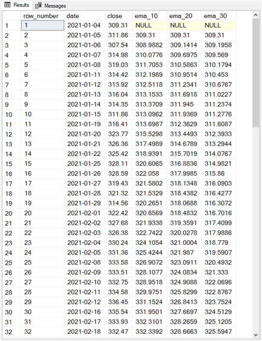
Here are the first thirty-two rows from the results set from the select statement at the end of the preceding script. You can compare this results set to the one at the end of the "A T-SQL example for computing simple moving averages" section to get a top line feel for some differences between simple moving averages and exponential moving averages.
- The table of exponential moving averages only has one row of missing values (null values). It is for the first row. The table of simple moving averages starts with 9, 19, and 29 missing rows, respectively, for the ten-period, twenty-period, and thirty-period simple moving averages.
- An even more important difference is the computational technique for the
two types of moving averages.
- Simple moving averages rely on the windows avg() function.
- There is no built-in T-SQL function for computing exponential moving averages. Furthermore, each exponential moving average depends on two different rows from the source data. Also, the value for the preceding row’s exponential moving average goes back to the second row of the source time series data. The row_number column values inside the while loop facilitate this behavior.
Selected empirical differences between simple and exponential moving averages
As you can see, there are different computational steps for computing simple and exponential moving averages. This section drills down on a pair of empirical differences between the two types of moving averages.
Which type of moving average values are closer to the underlying time series values?
The short answer to this question is the exponential moving average.
This tip computed simple and exponential moving averages for underlying time series values starting in January 2021 and running through May 2021. Moving averages were computed for three different period lengths for each of the two types of moving averages.
It is possible to compare each simple moving average and exponential moving average to its underlying time series value. The comparisons are performed with absolute values for the differences between a moving average and its underlying value. Because the simple moving averages start with 9, 19, and 29 null values, the number of possible comparisons changes for each period length.
- The number of comparison rows is 83 for 10-period comparisons, 73 for 20-period comparisons, and 63 for 30-period comparisons.
- The comparisons are to tell which type of moving average generates a smoothed value that is closer to the underlying value.
- For all three period lengths, the exponential moving averages are closer overall to the underlying time series values (71.087% of the comparisons for ten-period moving averages, 80.82% of the comparisons for twenty-period moving averages, and 88.89% of the comparisons for thirty-period moving averages).
This outcome is because the algorithm for exponential moving averages assigns progressively larger weights to the most recent underlying values in a time series. In contrast, the algorithm for simple moving averages assigns an equal weight to all underlying values inside the window for a period length. Additionally, the simple moving average algorithm excludes underlying values outside the window for a period length. Therefore, more underlying data values are excluded for shorter period lengths than longer period lengths.
| Comparison of exponential vs. simple moving averages for three different period lengths | |||
|---|---|---|---|
| 10-period results | 20-period results | 30-period results | |
| # of comparisons | 83 | 73 | 63 |
| # of exponential wins | 59 | 59 | 56 |
| % of exponential wins | 71.08 | 80.82 | 88.89 |
Do the moving averages change based on the start date?
The short answer is yes for exponential moving averages and no for simple moving averages. This type of question is common when comparing two sets of exponential moving averages for the same ending time period that start at different points in the past. For this sub-section, the tip created a second set of underlying time series values that started in January 2018 instead of January 2021.
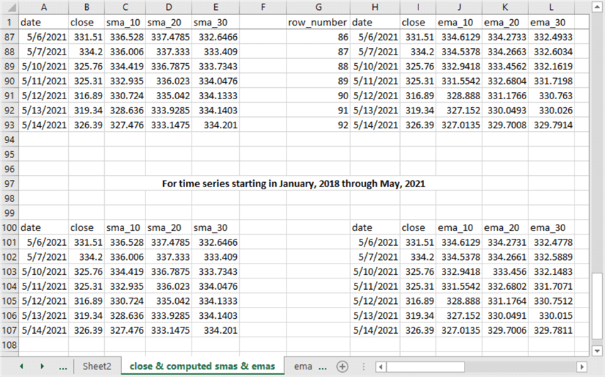
The following screen shot shows in its top set of rows the final seven close prices and moving averages for the set of underlying values starting in January 2021. The simple moving averages appear on the left, and the exponential moving averages appear on the right. The bottom set of rows shows close prices along with corresponding simple and exponential moving averages for underlying values starting in January 2018.
- As you can see, the simple moving average values are identical no matter whether the underlying time series starts in 2018 or 2021.
- In contrast, the exponential moving average values are not identical for underlying values starting in 2021 versus underlying values starting in 2018. While not identical, the values are approximately the same.
The reason for these differences is that the weights for the final seven dates are different depending on the start date. This is because there are two preceding years of weight applications for the exponential moving averages based on underlying values starting in 2018 versus the exponential moving averages based on underlying values starting in 2021. In contrast, the simple moving average just disregards all underlying values that are not in the current window of 10-periods, 20-periods, or 30-periods.
Next Steps
This tip’s download file contains three types of files to help you get a hands-on feel for computing simple and exponential moving averages for underlying time series values.
- There are two .csv files with different sets of underlying values.
- There are also two .sql files with code for computing simple moving averages and exponential moving averages.
- There is an Excel worksheet file with the sample data from 2021 for displaying and comparing simple and exponential moving averages.


About the author
 Rick Dobson is an author and an individual trader. He is also a SQL Server professional with decades of T-SQL experience that includes authoring books, running a national seminar practice, working for businesses on finance and healthcare development projects, and serving as a regular contributor to MSSQLTips.com. He has been growing his Python skills for more than the past half decade -- especially for data visualization and ETL tasks with JSON and CSV files. His most recent professional passions include financial time series data and analyses, AI models, and statistics. He believes the proper application of these skills can help traders and investors to make more profitable decisions.
This author pledges the content of this article is based on professional experience and not AI generated.
View all my tips