Optimizing Spark Performance with Adaptive Query Execution

By: Ron L'Esteve   |   Updated: 2021-09-23   |   Comments   |   Related: > Azure Databricks

Problem

While building out a Data Lakehouse, optimizing performance of big data workloads and queries are critical to the success and scalability of your production ready environment, in addition to maintaining high SLAs for business stakeholders that are frequently accessing data in the lake house. With all the robust performance enhancement capabilities of the more mature traditional SQL Data warehouses, it would be extremely valuable to have the capability of speeding up Spark SQL at runtime within a Data Lakehouse. Databricks has solved this with its Adaptive Query Execution (AQE) feature that is available with Spark 3.0 and higher. How can we get started with AQE, along with comparing performance of big data workloads in the Data Lakehouse with AQE both enabled and disabled?

Solution

The performance, maintainability, and scalability of a production ready Data Lakehouse environment is what truly determines its overall success. Traditional mature SQL Datawarehouse systems come with the benefits of indexing, statistics, automatic query plan optimizations and much more. The concept of the Data Lakehouse is slowly but surely maturing its capabilities and features when compared to many of these of these traditional systems. Adaptive Query Execution (AQE) is one such feature offered by Databricks for speeding up a Spark SQL query at runtime. In this article, I will demonstrate how to get started with comparing performance of AQE that is disabled versus enabled while querying big data workloads in your Data Lakehouse.

Part 1 – Comparing AQE Performance on Query without Joins

In an effort to diversify the sample demonstrations, this section will demonstrate how AQE performs on a dataset with approximately over 1 billion rows with no joins on the query. The exercise will compare the performance of AQE enabled versus disabled.

Pre-Requisites

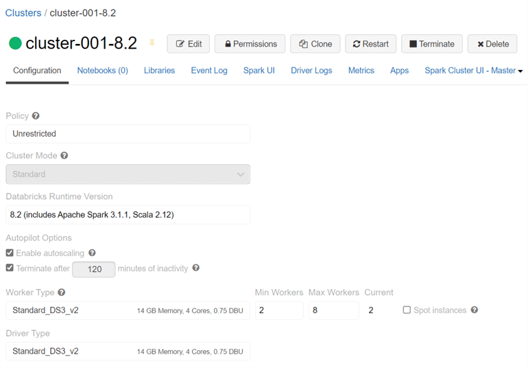
To begin, create a Databricks cluster similar to the one shown in the figure below. Notice that I have chosen relatively moderate worker and driver types, along with a runtime of 8.2 for this exercise. Obviously, the selected memory and cores will impact the query runtime so it is important to point out the configurations used for this exercise.

Create Dataset

Once the cluster has been created and started, go ahead and create a new SQL notebook; add and run the following Scala code, which will import the 2019 NYC Taxi yellow trip data set from databricks-datasets. The next part of the code will replicate the dataset 13 more times to create a much larger dataset containing over 1 billion rows. The final dataset will be saved to a data frame called nyctaxiDF.

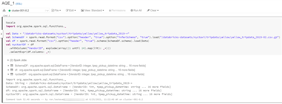
Here is the Scala code that you will need to run to import and replicate the 2019 NYC Taxi dataset and save to a data frame. Notice the explode function which performs the replication of data and can be customized to your desired data volume by simply changing the number 14 in the section which contains the following: explode(array((1 until 14).map(lit): _*))).

%scala
import org.apache.spark.sql.functions._
 
val Data = "/databricks-datasets/nyctaxi/tripdata/yellow/yellow_tripdata_2019-*"
val SchemaDF = spark.read.format("csv").option("header", "true").option("inferSchema", "true").load("/databricks-datasets/nyctaxi/tripdata/yellow/yellow_tripdata_2019-02.csv.gz")
val df = spark.read.format("csv").option("header", "true").schema(SchemaDF.schema).load(Data)
val nyctaxiDF = df
  .withColumn("VendorID", explode(array((1 until 14).map(lit): _*)))
  .selectExpr(df.columns: _*)

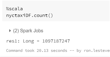
Run the following code to count the data frame to ensure that it contains the expected row count of over 1 billion rows.

Next, run the following Scala code which will write the nyctaxiDF to your ADLS gen2 account as Delta format. Please ensure that you have completed steps to mount your ADLS gen2 account within Databricks.

Here is the Scala code that your will need to run to write the nyctaxi data frame as Delta format to your ADLS gen2 account.

%scala
 
  val nyctaxiDF_delta = nyctaxiDF.write
  .format("delta")
  .mode("overwrite")
  .save("dbfs:/mnt/rcpdlhcore/datalakehouse/dlhcore/raw/delta/nyctaxi_A")

Once you have persisted the Delta format data to ADLS gen2, go ahead and run the following SQL command to create a Delta table using the location where you persisted the nyctaxi data frame within your ADLS gen2 account. You will be able to easily run SQL queries on your data using this Delta table.

Here is the SQL code that your will need to run to create the Delta table.

CREATE TABLE nyctaxi_A
USING DELTA 
LOCATION 'dbfs:/mnt/rcpdlhcore/datalakehouse/dlhcore/raw/delta/nyctaxi_A'

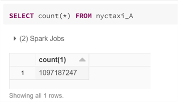
Run a count query to ensure that your newly created Delta table contains the expected count of over 1 billion rows in the table. Notice how you can easily run SQL queries on this the table, which demonstrates the ease of querying your Data Lakehouse using standard SQL syntax.

Disable AQE

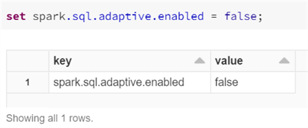
To test performance of AQE turned off, go ahead and run the following command to set spark.sql.adaptive.enabled = false;. This will ensure that AQE is switched off for this particular performance test.

Run the following SQL query in a new code block within your notebook to group and order by values within the table. Note that no joins have been included in this query at this point. Once the query completes running, notice that the command took 25.06 seconds to complete. This will be the benchmark time to test against once AQE is enabled for the same query. Because the query is applying groupings and orderings, the spark job will apply a shuffle / exchange and the default shuffle partitions are set to 200, which is why you will notice the stage with 200/200.

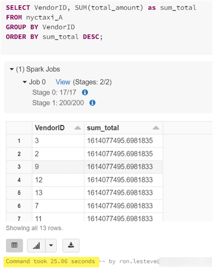
Here is the SQL query that you will need to run to test performance with AQE being disabled.

SELECT VendorID, SUM(total_amount) as sum_total
FROM nyctaxi_A
GROUP BY VendorID
ORDER BY sum_total DESC;

Enable AQE

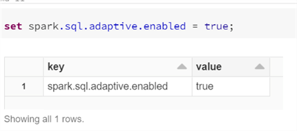
Next, go ahead and enable AQE by setting it to true with the following command: set spark.sql.adaptive.enabled = true;. In this section you'll run the same query provided in the previous section to measure performance of query execution time with AQE enabled.

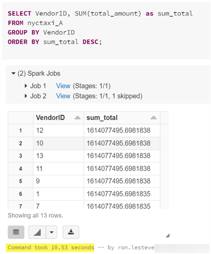
Once again, go ahead and run the same query again and notice that the command took 10.53 seconds this time with AQE enabled when compared to 25.06 seconds with AQE disabled; almost a 50% improvement in performance. Also, this time, the 200 stages were not executed in the Spark Jobs, which also demonstrates that AQE altered the plan at runtime.

In this section, you compared performance of the execution of a standard SQL query containing aggregations and joins on a large table containing over 1 billion rows.

Part 2 – Comparing AQE Performance on Query with Joins

Create Datasets

In this next section, create a new notebook and run the following code which is similar to Part 1, with the exception that we are also adding a new column to capture unique ids for each row. This unique id will be used to join two tables in the subsequent sections.

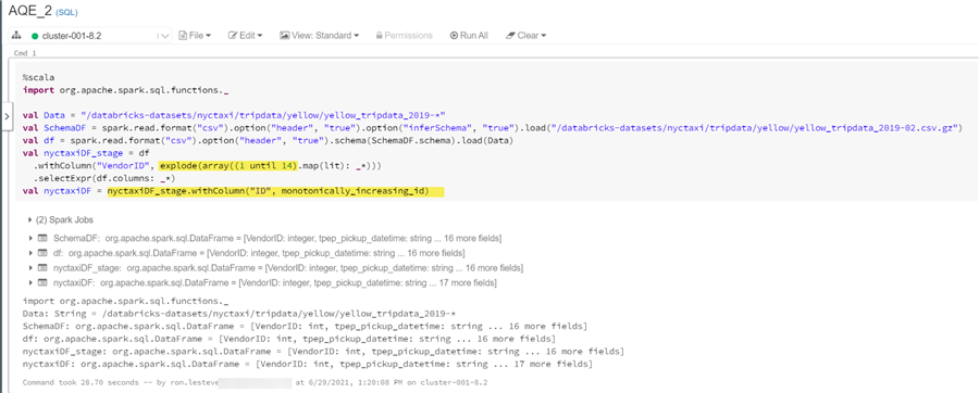
Here is the Scala code that you will need to run to generate the 2019 NYC Taxi dataset into a data frame. This code builds upon the code in the previous section with the addition of the ID column using 'monotonically_increasing_id'.

%scala
import org.apache.spark.sql.functions._
 
val Data = "/databricks-datasets/nyctaxi/tripdata/yellow/yellow_tripdata_2019-*"
val SchemaDF = spark.read.format("csv").option("header", "true").option("inferSchema", "true").load("/databricks-datasets/nyctaxi/tripdata/yellow/yellow_tripdata_2019-02.csv.gz")
val df = spark.read.format("csv").option("header", "true").schema(SchemaDF.schema).load(Data)
val nyctaxiDF_stage = df
  .withColumn("VendorID", explode(array((1 until 14).map(lit): _*)))
  .selectExpr(df.columns: _*)
val nyctaxiDF = nyctaxiDF_stage.withColumn("ID", monotonically_increasing_id)

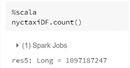
After running the code above, verify that the row counts of the data frame are as expected.

Run the following Scala code twice. For the first iteration, run the code with 'nyctaxi_A' specified in the file path. And for the second iteration, run the code with 'nyctaxi_B' specified in the file path. This will persist two large datasets, over 1 billion rows, in your specified ADLS gen2 folder path. These two datasets will be used to join to each other within a query.

%scala
 
  val nyctaxiDF_delta = nyctaxiDF.write
  .format("delta")
  .mode("overwrite")
  .save("dbfs:/mnt/rcpdlhcore/datalakehouse/dlhcore/raw/delta/nyctaxi_A")

Similarly, run the following SQL code twice, once for nyctaxi_A and the second for nyctaxi_B to create two Delta tables that you will use in query joins.

CREATE TABLE nyctaxi_A
USING DELTA 
LOCATION 'dbfs:/mnt/rcpdlhcore/datalakehouse/dlhcore/raw/delta/nyctaxi_A'

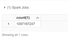
After creating the Delta tables, run a count, SELECT count(*) FROM nyctaxi_A, on both nyctaxi_A and nyctaxi_B to verify that they both contain over 1 billion rows.

You could also run a select statement to get a granular view of the data schema and structure. Also note that the newly created ID column auto increments unique ids for each row.

Disable AQE

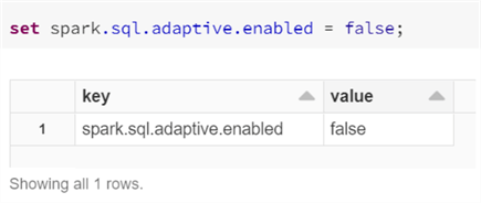
Similar to the previous section, go ahead and disable AQE for the first test by running the following command.

Here is the SQL query that joins the two Delta tables, applies a WHERE filter, GROUPs BY VendorID and ORDERs BY sum_total. The EXPLAIN FORMATTED command will describe the expected plan for this query before it is run.

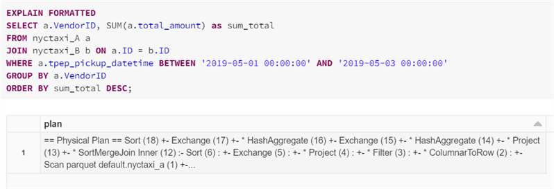
Here is the code that you will need to run to explain the physical plan of the SQL query.

EXPLAIN FORMATTED
SELECT a.VendorID, SUM(a.total_amount) as sum_total
FROM nyctaxi_A a
JOIN nyctaxi_B b ON a.ID = b.ID
WHERE a.tpep_pickup_datetime BETWEEN '2019-05-01 00:00:00' AND '2019-05-03 00:00:00'
GROUP BY a.VendorID
ORDER BY sum_total DESC;

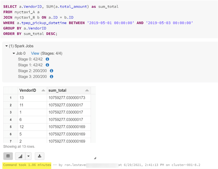
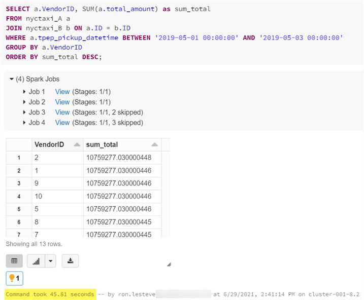
Next, run the following SQL query, which is simply the same query provided above with the exclusion of the EXPALIN FORMATTED command. Notice that there are 4 stages listed and the execution time took 1.06 minutes to complete. Since AQE is disabled, once again notice the additional stages containing the 200/200.

Enable AQE

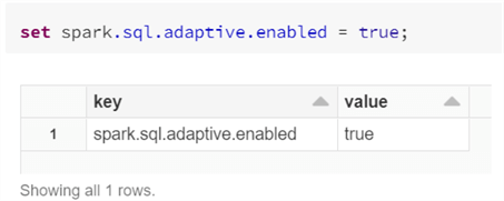
Next, go ahead and enable AQE by running the following command.

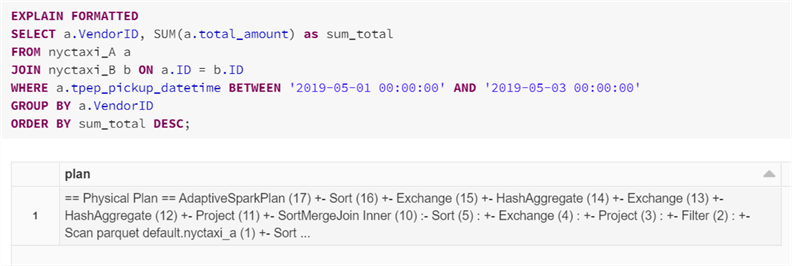
When you run the same code to explain the plan, you will notice that it generates the same plan and it did with AQE disabled. This is expected because AQE will adaptively change its query plan to a more optimized plan at run-time.

Run the same SQL query that was previously provided and notice that the execution time took only 45.81 seconds this time, which is a pretty significant improvement in performance due to the optimized AQE plan. Notice also that there were fewer stages as a result of AQE being enabled.

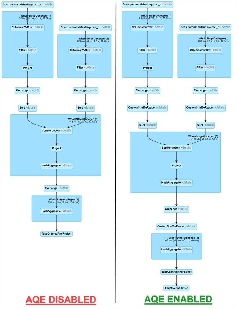
You can also dig into both of the query execution plans to compare and understand the differences between the plans with AQE was disabled and when it was enabled. This will also give you the opportunity to visually see where and how the AQE engine changed the plan during the execution of the query.

Summary

The AQE framework possesses the ability to 1) dynamically coalesce shuffle partitions, 2) dynamically switch join strategies, and 3) dynamically optimize skew joins. In this article, I introduced you to Adaptive Query Execution (AQE) and walked you through a real-world end to end example of comparing execution times of big data queries with AQE both enabled and disabled. In all scenarios, there were significant performance optimization gains and benefits with AQE being enabled. The capabilities of AQE demonstrate the performance optimization opportunities that contribute to advancing the adoption of the Data Lake house paradigm for production workloads.

Next Steps

• For more information on how the AQE Framework operates along with details about its feature sets, read How to Speed up SQL Queries with Adaptive Query Execution (databricks.com)
• For more information on analyzing and evolving query plans with AQE features, read Adaptive query execution | Databricks
• For other performance turning optimizations within Databricks, read Performance Tuning - Spark 3.1.2 Documentation (apache.org)

About the author

Ron L'Esteve is a trusted information technology thought leader and professional Author residing in Illinois. He brings over 20 years of IT experience and is well-known for his impactful books and article publications on Data & AI Architecture, Engineering, and Cloud Leadership. Ron completed his Master�s in Business Administration and Finance from Loyola University in Chicago. Ron brings deep tec

This author pledges the content of this article is based on professional experience and not AI generated.

View all my tips