Problem
Database pruning is an optimization process used to avoid reading files that do not contain the data that you are searching for. You can skip sets of partition files if your query has a filter on a particular partition column. In Apache Spark, Dynamic Partition Pruning is a capability that combines both logical and physical optimizations to find the dimensional filter, ensures that the filter executes only once on the dimension side, and then applies the filter directly to the scan of the table which speeds up queries and prevents reading unnecessary data. How can we get started with Dynamic Partition Pruning in Apache Spark?
Solution
Within Databricks, Dynamic Partition Pruning runs on Apache Spark compute and requires no additional configuration to be set to enable it. Fact tables which need to be pruned must be partitioned with join key columns and only work with equijoins. Dynamic Partition Pruning is best suited for optimizing queries that follow the Star Schema models. In this article, you will learn how to efficiently utilize Dynamic Partition Pruning in Databricks to run filtered queries on your Delta Fact and Dimension tables.
In the scenarios shown in the Figure below, without Dynamic Partition Pruning (DPP) applied, when you specify a filter on you date dimension that is joined to your fact table, all files will be scanned. Alternatively, with DPP applied, the optimizer will efficiently only prune the files that contain the relevant filter, assuming that your fact table is properly partitioned on the join key. Note that you can filter the query on a column within your date dimension that is not used in the join and it would still effectively partition prune the optimized query results.

For reference, here are a few Dynamic Partition Pruning commands and their descriptions. Most of these features are automatically enabled at the default settings, however it is still good to have an understanding of their capability through their description.
- spark.databricks.optimizer.dynamicFilePruning: (default is true) is the main flag that enables the optimizer to push down DFP filters.
- spark.databricks.optimizer.deltaTableSizeThreshold: (default is 10GB) This parameter represents the minimum size in bytes of the Delta table on the probe side of the join required to trigger dynamic file pruning.
- spark.databricks.optimizer.deltaTableFilesThreshold: (default is 1000) This parameter represents the number of files of the Delta table on the probe side of the join required to trigger dynamic file pruning.
To begin, ensure that you have created a cluster in your Databricks environment. For the purposes of this exercise, you can use a relatively small cluster, as shown in the figure below.

Once you have created the cluster, create a new Scala Databricks notebook and attach your cluster to this notebook. Also, ensure that your ADLS gen2 account is properly mounted. Run the following Python code shown in the figure below to check what mount points you have available: display(dbutils.fs.mounts())

Next, run the following Scala code shown in the figure below to import the 2019 NYC Taxi dataset into a data frame, apply schemas, and finally add Year, Month, Day derived columns to the data frame. These additional columns will be used to partition your Delta table in further steps of the process. Also, this dataset is available through ‘databricks-datasets’ in CSV form, which comes mounted to your cluster.

Here is the Scala code that you will need to run to load the 2019 NYCTaxi data into a data frame.
import org.apache.spark.sql.functions._
val Data = "/databricks-datasets/nyctaxi/tripdata/yellow/yellow_tripdata_2019-*"
val SchemaDF = spark.read.format("csv").option("header", "true").option("inferSchema", "true").load("/databricks-datasets/nyctaxi/tripdata/yellow/yellow_tripdata_2019-02.csv.gz")
val df = spark.read.format("csv").option("header", "true").schema(SchemaDF.schema).load(Data)
val nyctaxiDF = df
.withColumn("Year", year(col("tpep_pickup_datetime")))
.withColumn("Year_Month", date_format(col("tpep_pickup_datetime"),"yyyyMM"))
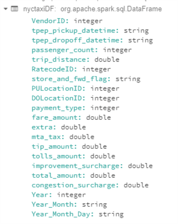
.withColumn("Year_Month_Day", date_format(col("tpep_pickup_datetime"),"yyyyMMdd"))After running the code, expand the data frame results to confirm that the schema in the expected format.
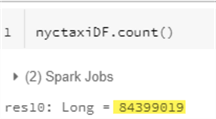
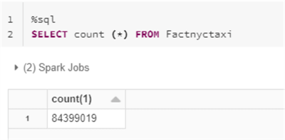
Run the following count of the data frame to ensure that there are ~84 million rows in the data frame.
Once the content of the data frame is finalized, run the following code to write the data to your desired ADLS gen2 mount point location; also add a partition by Year, Year_Month, and Year_Month_Day. It is these columns that you will use to join this fact table to your dimension table.

Here is the code that you will need to run to persist your NYCTaxi data in delta format to your ADLS gen2 account.
val Factnyctaxi = nyctaxiDF.write
  .format("delta")
  .mode("overwrite")
  .partitionBy(("Year"), ("Year_Month"), ("Year_Month_Day"))
  .save("/mnt/raw/delta/Factnyctaxi")
In addition to persisting the data frame to your ADLS gen2 account, also create a Delta SparkSQL Table using the SQL syntax below. With this table, you’ll be able to write standard SQL queries to join your fact and dimension tables in further sections.
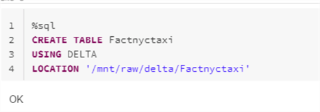
Here is the SQL code that you will need to run to create delta Spark SQL table.
%sql
CREATE TABLE Factnyctaxi
USING DELTA
LOCATION '/mnt/raw/delta/Factnyctaxi'
As a good practice, run a count of the newly created table to ensure that it contains the expected number of rows in the Factnyctaxi table.
As an added verification step, run the following SHOW PARTITIONS SQL command to confirm that the expected partitions have been applied to the Factnyctaxi table.

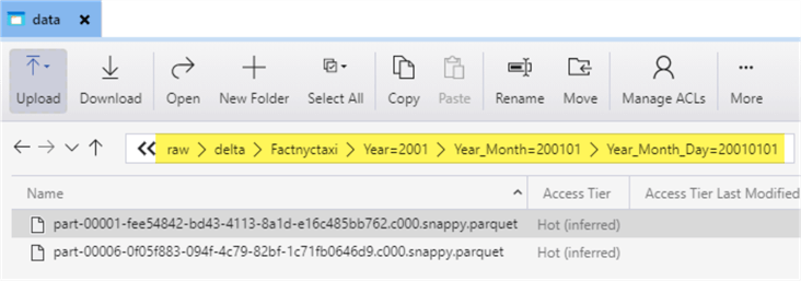
Upon navigating to the ADLS gen2 account through Storage Explorer, notice that the data is appropriately partitioned in the expected folder structure.
Similar to the process of creating the Factnyctaxi table, you will also need to create a dimension table. For this exercise, let’s create a date dimension table using the CSV file which can be downloaded from the following link: Date Dimension File – Sisense Support Knowledge Base. Upload this file to your ADLS gen2 account and then run the following script to load the csv file to a data frame.

Here is the code that you will need to run to infer the file’s schema and load the file to a data frame.
val dimedateDF = spark.read.format("csv")
.option("header", "true")
.option("inferSchema", "true")
.load("/mnt/raw/dimdates.csv")
Once the file is loaded to a data frame, run the following code to persist the data as delta format to your ADLS gen2 account.
val DimDate = dimedateDF.write
  .format("delta")
  .mode("overwrite")
  .save("/mnt/raw/delta/DimDate")
Also, execute the following SQL code to create a delta table called DimDate which will be joined to your Factnyctaxi table on a specified partition key.
%sql
CREATE TABLE DimDate
USING DELTA
LOCATION '/mnt/raw/delta/DimDate'
Run a SQL Select query to confirm that the date table was populated with data.

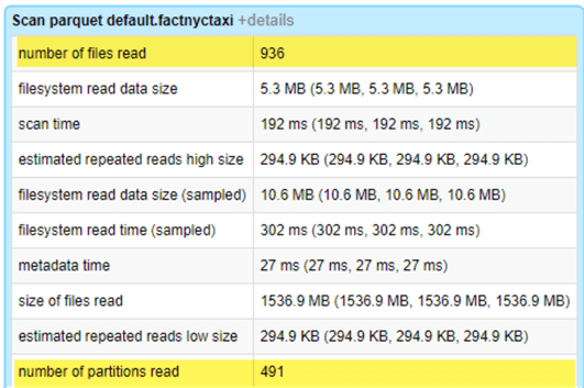
Run the following query which demonstrates a join of Factnyctaxi to DimDate on the Fact partitioned Year_Month_Day column for which the DateNum is the equivalent key in the DimDate table. Notice that a filter was not applied in this scenario to demonstrate from the execution plan that the Dynamic Partition Pruning will not be activate since there isn’t a filter that is being applied.

Here is the SQL query that you will need to run to generate the results shown in the figure above.
%sql
SELECT * FROM Factnyctaxi F
INNER JOIN DimDate D
ON F.Year_Month_Day = D.DateNum
From the query execution plan, notice the details of the scan of Factnyctaxi. The full 936 set of files were scan across all of the 491 partitions that were read. This indicates that since there was no filter applied, the dynamic partition pruning feature was not enabled for this scenario.
Run the following SQL query next. This query is similar to the previous one, with the addition of a where filter. Notice that this filter is not applied on any of the partition columns from Factnyctaxi, nor were they from the equivalent partition columns in DimDate. The filters that were applied were non join key columns in the dimension table.
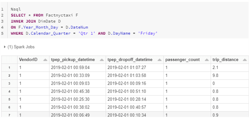
Here is the SQL query that you will need to run to generate the results shown in the figure above.
%sql
SELECT * FROM Factnyctaxi F
INNER JOIN DimDate D
ON F.Year_Month_Day = D.DateNum
WHERE D.Calendar_Quarter = 'Qtr 1' AND D.DayName = 'Friday'
From the query execution plan, notice the details of the scan of Factnyctaxi. Only 43 out of the full 936 set of files were scan across only 24 of the 491 partitions. Also notice that dynamic partition pruning has an execution time of 95ms, which indicates that dynamic partition pruning was applied to this query.

Summary
In this article, you learned about the various benefits of Dynamic Partition pruning along with how it is optimized for querying star schema models. This can be a valuable feature as you continue building out your Data Lakehouse in Azure. You also learned a hands-on technique for re-creating a scenario best suited for dynamic partition pruning by joining a fact and dimension table on a partition key column and filtering the dimension table on a non-join key. Upon monitoring the query execution plan for this scenario, you learned that dynamic partition pruning had been applied and a significantly smaller subset of the data and partitions were read and scanned.
Next Steps
- For more details on Dynamic Partition Pruning, see Spark 3.0 Feature — Dynamic Partition Pruning (DPP) to avoid scanning irrelevant Data.
- To learn more about Dynamic Partition Pruning, its benefits, along with real world examples, see How to optimize and increase SQL query speed on Delta Lake – The Databricks Blog.
- For more information on Dynamic Partition Pruning in video form, see Dynamic Partition Pruning in Apache Spark – Databricks

Ron C. L’Esteve is a Data and AI Leader and professional Author residing in Chicago, IL, USA. He is well-known for his impactful books and article publications on Azure Data & AI Architecture, Engineering, and Leadership. Ron holds a Master of Business Administration (M.B.A.) and Master of Science in Corporate Finance (M.S.F.) from Loyola University Chicago. Ron possesses deep technical skills and experience in designing, implementing, leading, and delivering modern Azure Data & AI projects for numerous clients around the world. He is a Motorola Certified Six Sigma Green Belt, a Microsoft Global Challenger, and also holds numerous additional Microsoft, Snowflake, and Databricks professional certifications in Big Data Engineering, Artificial Intelligence, Apache Spark and Data Platform Architecture.
- MSSQLTips Awards: Champion (100+ tips) – 2023 | Author of the Year – 2020-2021 | Rookie of the Year – 2019