SQL Aggregate Functions in SQL Server, Oracle and PostgreSQL

Problem

In the first part of this tip series, SQL Aggregate Functions in SQL Server, Oracle and PostgreSQL, we have seen the basic features of aggregate functions, with an overview of the most used and options such as GROUP BY and DISTINCT. In this SQL tutorial, we look at some additional aggregate functions and how the differ between SQL Server, Oracle and PostgreSQL.

Solution

In this second part we will dig a little more into the topic, introducing HAVING, the use of aggregates with OVER clause, different classifications of functions in Oracle and some other differences in PostgreSQL.

As always, we will use the GitHub freely downloadable database sample Chinook, as it is available in multiple RDBMS formats. It is a simulation of a digital media store, with some sample data, all you have to do is download the version you need and you have all the scripts for data structure and all the Inserts for data.

Let's take a look at the first topic, as you may know it is possible to add a filter using the aggregate function, this is done with the HAVING clause.

SQL Server

It is possible to filter the grouped data set in order to retrieve a specific group of data in a SQL database. For example, suppose that we need to extract only the customers that have been invoiced at least 40 dollars along with the total number of invoices with this SELECT statement:

select invoice.CustomerId,
       firstname + ' ' + lastname as Customer, 
       count(invoiceid) as num_invoices, -- COUNT Function 
       sum(total) as Total_amount
from Invoice
inner join Customer on invoice.CustomerId=Customer.CustomerId
group by invoice.CustomerId, firstname + ' ' + LastName
having sum(total) >= 40;

Very simple way to filter just the highest sales in a SQL statement.

Obviously HAVING clauses can be combined using AND/OR and it is possible to use them in CTEs like I did in this nice example in the UPDATE (and also INSERT) tip: SQL Update Statement with Join in SQL Server vs Oracle vs PostgreSQL.

; with discount as
( select Invoice.CustomerId, sum(invoiceline.UnitPrice*Quantity) as genretotal
  from invoice
  inner join InvoiceLine on Invoice.InvoiceId=InvoiceLine.InvoiceId
  inner join Track on Track.TrackId=InvoiceLine.TrackId
  inner join customer on customer.CustomerId=Invoice.CustomerId
  where country = 'Austria' and GenreId in (1,3) -- WHERE Clause
  group by Invoice.CustomerId
  having sum(invoiceline.UnitPrice*Quantity) > 20
)
update Invoice
set total=total*0.8
from Invoice
inner join discount on Invoice.CustomerId=discount.CustomerId

In this case, the example is applying a 20% discount using a CTE in order to extract the specific invoices with more than 20 USD spent on Rock and Metal for Austrian customers, making use of the HAVING clause for this purpose.

Now let's spice up our game and see another topic that I introduced in a past tip: the OVER clause.

As I showed in the tip on windowing functions, SQL Window Functions in SQL Server, Oracle and PostgreSQL, the OVER clause is used together with aggregate functions or statistical functions in order to aggregate based not on a GROUP BY, but across a number of rows, a sliding subset of data like a window on a data set.

Let me demonstrate it with another SELECT statement example, different from the ones on the windowing functions tip and focused on aggregate functions in the following query. Let's suppose that we want the breakdown of invoices aggregated by invoice number and genre:

select distinct
   Invoiceid, genre.[Name], 
   sum(Quantity*invoiceline.UnitPrice) over (partition by invoiceid) as TotalInvoice, -- SELECT SUM
   sum(Quantity*invoiceline.UnitPrice) over (partition by invoiceid, genre.name) as TotalInvoice_genre, -- SELECT SUM
   count(invoicelineid) over (partition by invoiceid) as TotalRows, -- SELECT COUNT Function
   count(invoicelineid) over (partition by invoiceid, genre.name) as TotalRows_genre, -- SELECT COUNT Function
   max(quantity) over (partition by invoiceid) as MaxQuantity, -- Maximum Value with SELECT MAX
   min(quantity) over (partition by invoiceid) as MinQuantity -- Minimum Value with SELECT MIN
from InvoiceLine
inner join Track on InvoiceLine.TrackId=Track.TrackId
inner join Genre on Track.GenreId=Genre.GenreId

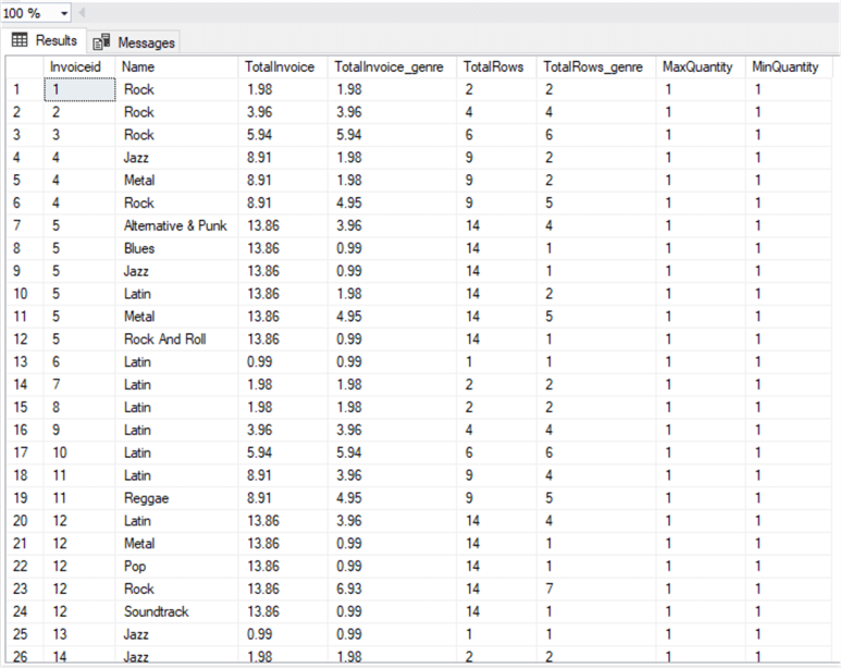
In this way, we've obtained in the same query both the totals per invoice and the breakdown aggregated per invoice/genre, adding also a maximum and minimum quantity on the invoice, just using different OVER (PARTITION BY) clauses. A lot easier and efficient than doing subqueries or CTEs! Pay attention that if PARTITION BY is omitted, then the aggregation functions are applied on all rows returned by the query.

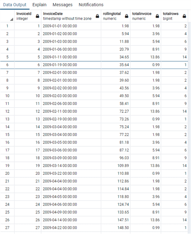
With OVER we can use also ORDER BY, in combination with PARTITION BY or alone, let's do another example:

select distinct invoiceline.invoiceid, -- Distinct Values
   invoicedate,
   sum(Quantity*invoiceline.UnitPrice) over (order by invoiceline.invoiceid) as RollingTotal, -- SUM Function
   sum(Quantity*invoiceline.UnitPrice) over (partition by invoiceline.invoiceid order by invoicedate) as TotalInvoice, -- SUM Function
   count(invoicelineid) over (partition by invoiceline.invoiceid) as TotalRows
from InvoiceLine
inner join Track on InvoiceLine.TrackId=Track.TrackId
inner join invoice on invoiceline.invoiceid=invoice.invoiceid

As you can see with the first aggregation, we've obtained the rolling total so a total of invoices incremented with each invoice ordered by invoice id, the second is the total of the invoice as we've partitioned by invoiceid and ordered by invoice date (this later order by is redundant as the invoice ids are already in the same order). Last, we have a count of the invoice lines having partitioned by invoiceid like in the previous query. Easy and very powerful, isn't it?

It is common to see together with aggregation functions in OVER() clauses the use of analytic and rank functions as I showed in some examples in the windowing functions tip. The most common are LAG, LEAD, FIRST_VALUE and LAST_VALUE for the analytic and RANK and ROW_NUMBER for the rank. These have a different classification in SQL Server, so they are not considered aggregate functions which is different in Oracle.

But first let me do another example using aggregate, analytic and rank functions:

; with total_genre as
(select genre.name as genre, sum(Quantity*invoiceline.UnitPrice) as TotalInvoice_genre
from InvoiceLine
inner join Track on InvoiceLine.TrackId=Track.TrackId
inner join Genre on Track.GenreId=Genre.GenreId
group by genre.name)
select genre, rank() over (order by totalinvoice_genre desc) as ranking, FIRST_VALUE(genre) over(order by totalinvoice_genre desc) as First_Place
from total_genre

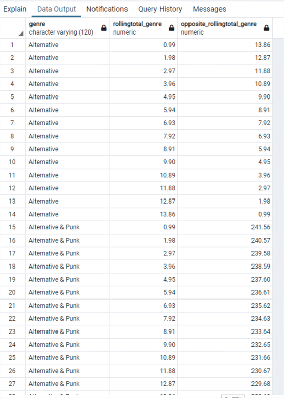
Here is a very simple example of RANK() and FIRST_VALUE() functions used together in order to retrieve the ranking of sales by genre and reminding also which one is in first place, using a CTE in order to obtain the total invoiced per genre.

There is another example with OVER() clause using aggregate functions that I'd like to present, as I didn't write about it in my windowing functions tip: specifying the ROWS or RANGE, thus limiting the window of rows evaluated within a partition. Please refer to the official documentation for a very good explanation of that concept: https://docs.microsoft.com/en-us/sql/t-sql/queries/select-over-clause-transact-sql?view=sql-server-ver15.

And let's do a practical example:

select distinct genre.name as Genre,
   sum(Quantity*invoiceline.UnitPrice) over (partition by genre.name order by invoicedate ROWS UNBOUNDED PRECEDING) as RollingTotal_Genre,
   sum(Quantity*invoiceline.UnitPrice) over (partition by genre.name order by invoicelineid ROWS between current row and UNBOUNDED following) as Opposite_RollingTotal_Genre
from InvoiceLine
inner join Track on InvoiceLine.TrackId=Track.TrackId
inner join Genreon Track.GenreId=Genre.GenreId
inner join invoice on invoiceline.invoiceid=invoice.invoiceid

In this query I have defined two different windows range of rows using ROWS UNBOUNDED PRECEDING and FOLLOWING, the first returns the rolling total by genre, the second does the same but as a sort of a countdown. Specifying UNBOUNDED PRECEDING means that the range is between the current row and all preceding rows, thus giving us the rolling total so far, instead the second defines the range between the current row and all following.

Oracle

Let's start seeing how HAVING behaves in Oracle, doing the same query as in SQL Server:

select invoice.CustomerId,firstname||' '||LastName as Customer, count(invoiceid) as num_invoices, 
       sum(total) as Total_amount
from chinook.Invoice
inner join chinook.Customer
on invoice.CustomerId=Customer.CustomerId
group by invoice.CustomerId,firstname||' '||LastName
having sum(total)>=40;

As you can see, we have the same exact behavior as in SQL Server, using HAVING is ANSI standard.

The same combinations of HAVING that I described before on SQL Server are valid in Oracle, if you recall the example done in the tip about UPDATEs with JOINs, I did the example on Oracle using MERGE:

MERGE INTO chinook.Invoice
USING 
 ( select Invoice.CustomerId as customerid_sub, sum(invoiceline.UnitPrice*Quantity) as genretotal
   from chinook.invoice
   inner join chinook.InvoiceLine on Invoice.InvoiceId=InvoiceLine.InvoiceId
   inner join chinook.Track on Track.TrackId=InvoiceLine.TrackId
   inner join chinook.customer on customer.CustomerId=Invoice.CustomerId
   where country='Austria' and GenreId in (1,3)
   group by Invoice.CustomerId
   having sum(invoiceline.UnitPrice*Quantity)>20
  ) 
ON (Invoice.CustomerId=Customerid_sub)
WHEN MATCHED THEN
UPDATE set total=total*0.8;

As you can see, we have basically the same syntax as in SQL Server regarding the HAVING clause.

Let's do the same example we did before in SQL Server with the OVER clause:

select distinct
   Invoiceid, Genre.Name, 
   sum(Quantity*invoiceline.UnitPrice) over (partition by invoiceid) as TotalInvoice,
   sum(Quantity*invoiceline.UnitPrice) over (partition by invoiceid, genre.name) as TotalInvoice_genre,
   count(invoicelineid) over (partition by invoiceid) as TotalRows,
   count(invoicelineid) over (partition by invoiceid, genre.name) as TotalRows_genre,
   max(quantity) over (partition by invoiceid) as MaxQuantity,
   min(quantity) over (partition by invoiceid) as MinQuantity
from chinook.InvoiceLine
inner join chinook.Track on InvoiceLine.TrackId=Track.TrackId
inner join chinook.Genre on Track.GenreId=Genre.GenreId;

Again, we have the same syntax but not the same result as in SQL Server, in fact the order is not the same as in SQL Server, but this should be expected as we all know that we cannot say that a data set is ordered unless we explicitly apply an ORDER BY. So, in this case if we want to have the same result we must apply an ORDER BY:

select distinct
Invoiceid, Genre.Name, 
sum(Quantity*invoiceline.UnitPrice) over (partition by invoiceid) as TotalInvoice,
sum(Quantity*invoiceline.UnitPrice) over (partition by invoiceid, genre.name) as TotalInvoice_genre,
count(invoicelineid) over (partition by invoiceid) as TotalRows,
count(invoicelineid) over (partition by invoiceid, genre.name) as TotalRows_genre,
max(quantity) over (partition by invoiceid) as MaxQuantity,
min(quantity) over (partition by invoiceid) as MinQuantity
from chinook.InvoiceLine
inner join chinook.Track on InvoiceLine.TrackId=Track.TrackId
inner join chinook.Genre on Track.GenreId=Genre.GenreId
ORDER BY invoiceid;

And now let's do the example applying the ORDER BY to the OVER clause as in SQL Server in this case we also need to apply the same order by to the result data set otherwise we end up with a wrong result:

select distinct invoiceline.invoiceid, invoicedate,
   sum(Quantity*invoiceline.UnitPrice) over (order by invoiceline.invoiceid) as RollingTotal, 
   sum(Quantity*invoiceline.UnitPrice) over (partition by invoiceline.invoiceid order by invoicedate) as TotalInvoice,
   count(invoicelineid) over (partition by invoiceline.invoiceid) as TotalRows
from chinook.InvoiceLine
inner join chinook.Track on InvoiceLine.TrackId=Track.TrackId
inner join chinook.invoice on invoiceline.invoiceid=invoice.invoiceid
order by invoiceid;

So far, except the order of the data set, we have not encountered any difference between SQL Server and Oracle, but let's talk about analytic and rank functions: as I hinted above. In Oracle these last two are classified and considered as aggregate functions if you check the official documentation.

Moreover, you'll find another interesting thing in the same documentation referring to aggregate functions:

"Some aggregate functions allow the windowing_clause, which is part of the syntax of analytic functions. Refer to windowing_clause for information about this clause. In the listing of aggregate functions at the end of this section, the functions that allow the windowing_clause are followed by an asterisk (*)"

What is this windowing clause? Why does it say that only some of the aggregation functions allow it? Has it something to do with the windowing functions explained in one of my previous tips?

The answer is simple, it is the same as the ROWS/RANGE clause in SQL Server, used in the OVER() clause to define a window over which the rows are evaluated as I showed in the last example in SQL Server. In Oracle it's called a windowing clause even if it has the same syntax, moreover using the OVER clause in Oracle is considered using analytic functions, not aggregate functions, that's why following that link of windowing_clause will point you to the analytic functions documentation.

Let's do first the same example as in SQL Server with RANK() and then with the windowing clause:

with total_genre as
(select genre.name as genre, sum(Quantity*invoiceline.UnitPrice) as TotalInvoice_genre
from chinook.InvoiceLine
inner join chinook.Track on InvoiceLine.TrackId=Track.TrackId
inner join chinook.Genre on Track.GenreId=Genre.GenreId
group by genre.name)
select genre, rank() over (order by totalinvoice_genre desc) as ranking, FIRST_VALUE(genre) over(order by totalinvoice_genre desc) as First_Place
from total_genre;

Exactly the same as in SQL Server, now the example with the windowing function:

select distinct genre.name as Genre,
   sum(Quantity*invoiceline.UnitPrice) over (partition by genre.name order by invoicedate ROWS UNBOUNDED PRECEDING) as RollingTotal_Genre,
   sum(Quantity*invoiceline.UnitPrice) over (partition by genre.name order by invoicelineid ROWS between current row and UNBOUNDED following) as Opposite_RollingTotal_Genre
from chinook.InvoiceLine
inner join chinook.Track on InvoiceLine.TrackId=Track.TrackId
inner join chinook.Genre on Track.GenreId=Genre.GenreId
inner join chinook.invoice on invoiceline.invoiceid=invoice.invoiceid
order by genre.name;

Again, in Oracle we need to specify the Order By to retrieve the same result, but the syntax of the windowing clause is the same as SQL Server.

PostgreSQL

In PostgreSQL we have the same HAVING clause as the other two RDBMS, so let's do the first example:

select "Invoice"."CustomerId","FirstName"||' '||"LastName" as customer, count("InvoiceId") as num_invoices, 
       sum("Total") as total_amount
from "Invoice"
inner join "Customer"
on "Invoice"."CustomerId"="Customer"."CustomerId"
group by "Invoice"."CustomerId","FirstName"||' '||"LastName"
having sum("Total")>=40;

Again, we have the same syntax, now the same example done in the tip on UPDATE with joins:

; with discount as
( select "Invoice"."CustomerId", sum("InvoiceLine"."UnitPrice"*"Quantity") as genretotal
  from "Invoice" 
  inner join "InvoiceLine" on "Invoice"."InvoiceId"="InvoiceLine"."InvoiceId"
  inner join "Track" on "Track"."TrackId"="InvoiceLine"."TrackId"
  inner join "Customer" on "Customer"."CustomerId"="Invoice"."CustomerId"
  where "Country"='Austria' and "GenreId" in (1,3)
  group by "Invoice"."CustomerId"
  having sum("InvoiceLine"."UnitPrice"*"Quantity")>20
 )
update "Invoice"
set "Total"="Total"*0.8
from discount
where "Invoice"."CustomerId"=discount."CustomerId";

Which is the same syntax as in SQL Server.

Now let's do the examples with the OVER clause:

select distinct
   "InvoiceId", "Genre"."Name", 
   sum("Quantity"*"InvoiceLine"."UnitPrice") over (partition by "InvoiceId") as totalinvoice,
   sum("Quantity"*"InvoiceLine"."UnitPrice") over (partition by "InvoiceId", "Genre"."Name") as totalinvoice_genre,
   count("InvoiceLineId") over (partition by "InvoiceId") as totalrows,
   count("InvoiceLineId") over (partition by "InvoiceId", "Genre"."Name") as totalrows_genre,
   max("Quantity") over (partition by "InvoiceId") as MaxQuantity,
   min("Quantity") over (partition by "InvoiceId") as MinQuantity
from "InvoiceLine"
inner join "Track" on "InvoiceLine"."TrackId"="Track"."TrackId"
inner join "Genre" on "Track"."GenreId"="Genre"."GenreId";

We have the same behavior as in Oracle, so we need to explicitly order the result set:

select distinct
   "InvoiceId", "Genre"."Name", 
   sum("Quantity"*"InvoiceLine"."UnitPrice") over (partition by "InvoiceId") as totalinvoice,
   sum("Quantity"*"InvoiceLine"."UnitPrice") over (partition by "InvoiceId", "Genre"."Name") as totalinvoice_genre,
   count("InvoiceLineId") over (partition by "InvoiceId") as totalrows,
   count("InvoiceLineId") over (partition by "InvoiceId", "Genre"."Name") as totalrows_genre,
   max("Quantity") over (partition by "InvoiceId") as MaxQuantity,
   min("Quantity") over (partition by "InvoiceId") as MinQuantity
from "InvoiceLine"
inner join "Track" on "InvoiceLine"."TrackId"="Track"."TrackId"
inner join "Genre" on "Track"."GenreId"="Genre"."GenreId"
order by "InvoiceId";

And now the example with the order by in the OVER clause:

select distinct "InvoiceLine"."InvoiceId", "InvoiceDate",
   sum("Quantity"*"InvoiceLine"."UnitPrice") over (order by "InvoiceLine"."InvoiceId") as RollingTotal, 
   sum("Quantity"*"InvoiceLine"."UnitPrice") over (partition by "InvoiceLine"."InvoiceId" order by "InvoiceDate") as TotalInvoice,
   count("InvoiceLineId") over (partition by "InvoiceLine"."InvoiceId") as TotalRows
from "InvoiceLine"
inner join "Track" on "InvoiceLine"."TrackId"="Track"."TrackId"
inner join "Invoice" on "InvoiceLine"."InvoiceId"="Invoice"."InvoiceId"
order by "InvoiceId";

Again, same behavior as in Oracle so we need to explicitly order by invoiceid.

Finally let's review some of the different classifications of functions in PostgreSQL: as per the official documentation the last examples I presented with the OVER clause are not to be considered as aggregate functions but window functions. There are aggregate functions, but then also aggregate functions for statistics with obviously specific calculus related functions. Then we have Ordered Set aggregate functions and Hypothetical – Set aggregate functions: these are included with the RANK and DENSE_RANK, see documentation link and documentation on window functions.

So, let's do the last example with RANK and windowing ranges!

with total_genre as
(select "Genre"."Name" as genre, sum("Quantity"*"InvoiceLine"."UnitPrice") as TotalInvoice_genre
from "InvoiceLine"
inner join "Track" on "InvoiceLine"."TrackId"="Track"."TrackId"
inner join "Genre" on "Track"."GenreId"="Genre"."GenreId"
group by "Genre"."Name")
select genre, rank() over (order by totalinvoice_genre desc) as ranking, FIRST_VALUE(genre) over(order by totalinvoice_genre desc) as First_Place
from total_genre;

And now the window function:

select distinct "Genre"."Name" as genre,--"InvoiceLine"."InvoiceId", "InvoiceLine"."InvoiceLineId", 
   sum("Quantity"*"InvoiceLine"."UnitPrice") over (partition by "Genre"."Name" order by "InvoiceDate" ROWS UNBOUNDED PRECEDING) as RollingTotal_Genre,
   sum("Quantity"*"InvoiceLine"."UnitPrice") over (partition by "Genre"."Name" order by "InvoiceLineId" ROWS between current row and UNBOUNDED following) as Opposite_RollingTotal_Genre
from "InvoiceLine"
inner join "Track" on "InvoiceLine"."TrackId"="Track"."TrackId"
inner join "Genre" on "Track"."GenreId"="Genre"."GenreId"
inner join "Invoice" on "InvoiceLine"."InvoiceId"="Invoice"."InvoiceId"
order by genre;

And here we have a totally mixed-up result! It happens that making use of the DISTINCT clause (that in this query is totally unnecessary) the order is mixed up, so if we omit it:

select "Genre"."Name" as genre,
   sum("Quantity"*"InvoiceLine"."UnitPrice") over (partition by "Genre"."Name" order by "InvoiceDate" ROWS UNBOUNDED PRECEDING) as RollingTotal_Genre,
   sum("Quantity"*"InvoiceLine"."UnitPrice") over (partition by "Genre"."Name" order by "InvoiceLineId" ROWS between current row and UNBOUNDED following) as Opposite_RollingTotal_Genre
from "InvoiceLine"
inner join "Track" on "InvoiceLine"."TrackId"="Track"."TrackId"
inner join "Genre" on "Track"."GenreId"="Genre"."GenreId"
inner join "Invoice" on "InvoiceLine"."InvoiceId"="Invoice"."InvoiceId"
order by genre;

And formally this is the most correct result of the three RDBMS!

Conclusions

In this second part of the tip dedicated to aggregate functions, we have seen the use of HAVING and OVER clauses, the differences in classifications of aggregate functions in the three RDBMS and the different results determined by the usage of ORDER BY and DISTINCT.

Next Steps

About the author

Andrea Gnemmi is a Database and Data Warehouse professional with almost 20 years of experience, having started his career in Database Administration with SQL Server 2000.

This author pledges the content of this article is based on professional experience and not AI generated.

View all my tips

Article Last Updated: 2022-06-27

SQL Aggregate Functions Having, Order By, Distinct, Partition By and more in SQL Server, Oracle and PostgreSQL