Python Functions - Median, Quantiles, Variance, STDev and Correlation

By: Hristo Hristov | Updated: 2022-07-27 | Comments | Related: > Python

Problem

In a previous tip, we laid the groundwork of how to develop basic statistical functions with Python. Consequently, the purpose of this tip is to expand this topic by showing examples of built-in, ready-to-use functions as compared to examples written from scratch. The additional goal here is to demonstrate how to use these statistical functions with real data coming from SQL Server.

Solution

Python provides an additional module called statistics. It gives you quick and convenient access to ready-made functions so you can calculate several types of measures of central location (i.e., averages), measures of spread (i.e., variance and standard deviation), as well as the relation between two sets of data (i.e., covariance and correlation).

Environment

In case you have not yet please read my tip on How to Get Started Using Python Using Anaconda and VS Code. Then, open VS Code in your working directory. Create a new file with the .ipynbextension:

Next, open your file by double-clicking on it and select a kernel:

You will get a list of all your conda environments and any default interpreters if such are installed. You can pick an existing interpreter or create a new environment from the conda interface or terminal prior. Install the following modules additionally:

pandas by running pip install pandas
sqlalchemy by running pip install SQLAlchemy in the terminal of your environment.

Next, import the installed modules and the statistics package (which comes bundled with your Python interpreter but requires an import). Finally, create an SQL connection with the create_engine method (as shown in a previous tip):

import pandas as pd
from sqlalchemy import create_engine
import statistics as st
 
engine = create_engine(
    'mssql+pyodbc://'
    '@./AdventureWorksDW2019?'  # username:pwd@server:port/database
    'driver=ODBC+Driver+17+for+SQL+Server'
)

Example data

We will apply the statistics functions on data from AdventureWorksDW2019. Head over to this place for instructions on how to restore the database from backup. Alternatively, you can use your own database provided you generate dataframes compatible with the statistical functions.

Median

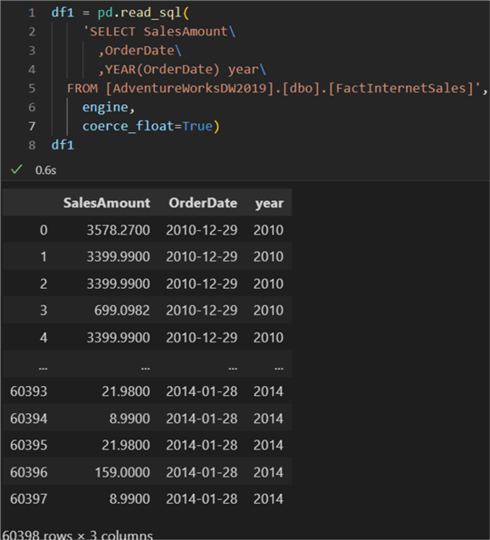
Let us imagine we need the median sales values per year. First, we must construct a query, then pass it to the pandas read_sql method so the result is a ready-to-work-with dataframe:

df1 = pd.read_sql(
    'SELECT SalesAmount\
      ,OrderDate\
      ,YEAR(OrderDate) year\
  FROM [AdventureWorksDW2019].[dbo].[FactInternetSales]',
    engine,
    coerce_float=True)

Next, we must aggregate per year and take the median. There is a pandas way to do that or you can do it from the query itself. In this case, we will highlight the way to do it manually. First, we get all distinct years. We also need an empty dictionary to store the results. Inside the loop, for each year, we calculate the current sales (resulting in a dataframe) and pass that dataframe to the median function. The keys will be each year and the value will be the median sales amount in USD:

years = df1.year.unique()
means = {}
for year in years:
    current_year_sales = df1[df1.year==year].SalesAmount # performs filter per year and takes only               
                                                         # the sales amount
    current_mean = st.median(current_year_sales)
    means[year]= current_mean

The result shows the evolution of the median of sales per year. The last two years have had unusually low values due to low sales.

Quantiles

To further our analysis of the sales amounts, let us also look at making quantiles and separating the values into those quantiles. Here we can use the quantiles method. It needs two arguments: the dataframe and the number of intervals to divide the data. The default is 4 for quartiles but let us use 10 for deciles:

dec = st.quantiles(df1.SalesAmount, n = 10)

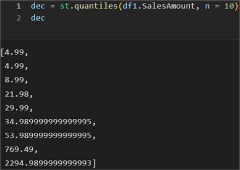
The result is 9 values which denote the cut points of the 10 intervals. Each interval represents 1/10 of the sample data.

Variance and Standard Deviation

Next, let us imagine we needed to take the variance and standard deviation of the sales amount per country. This will give us an idea of how far from the average the values are dispersed. This is the proposed query that returns all-time sales per country:

df2 = pd.read_sql(
    'SELECT st.SalesTerritoryCountry,\
        f.SalesAmount\
  FROM [AdventureWorksDW2019].[dbo].[FactInternetSales] as f\
  JOIN DimSalesTerritory as st ON f.SalesTerritoryKey = st.SalesTerritoryKey',
    engine,
    coerce_float=True)
df2

Next, we can follow along the same logic as for the median calculation: extract the distinct country names, filter the sales out per country, and store the variance and standard deviation values in a dictionary:

countries = df2.SalesTerritoryCountry.unique()
var_country = {}
for country in countries:
    current_country_sales = df2[df2.SalesTerritoryCountry==country].SalesAmount
    current_var = st.variance(current_country_sales)
    current_std = st.stdev(current_country_sales)
    var_country[country]= (current_var, current_std)
var_country

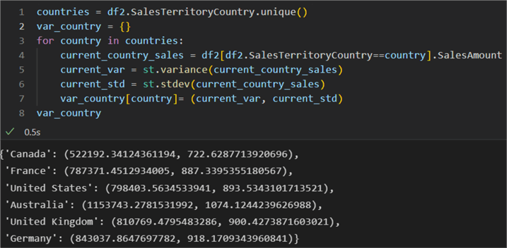
calculating variance and stdev per country

As expected, for each country we have a tuple holding the variance and the standard deviation value.

Correlation

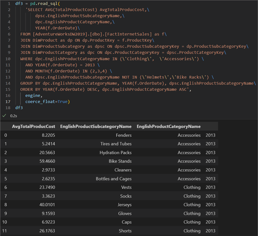
Finally, with the statistics package, it is quite straightforward to find the correlation between a pair of inputs. The only requirement is for the inputs to be of the same size. For example, let us execute a query which returns the average total product cost per product category for the year 2013:

df3 = pd.read_sql(
    'SELECT AVG(TotalProductCost) AvgTotalProducCost,\
        dpsc.EnglishProductSubcategoryName,\
        dpc.EnglishProductCategoryName,\
        YEAR(f.OrderDate)\
  FROM [AdventureWorksDW2019].[dbo].[FactInternetSales] as f\
  JOIN DimProduct as dp ON dp.ProductKey = f.ProductKey\
  JOIN DimProductSubcategory as dpsc ON dpsc.ProductSubcategoryKey = dp.ProductSubcategoryKey\
  JOIN DimProductCategory as dpc ON dpc.ProductCategoryKey = dpsc.ProductCategoryKey\
  WHERE dpc.EnglishProductCategoryName IN (\'Clothing\',  \'Accessories\') \
    AND YEAR(f.OrderDate) = 2013 \ # can be a parameter elsewhere in the code 
    AND MONTH(f.OrderDate) IN (2,3,4) \ 
    AND dpsc.EnglishProductSubcategoryName NOT IN (\'Helmets\',\'Bike Racks\') \
  GROUP BY dpc.EnglishProductCategoryName, YEAR(f.OrderDate), dpsc.EnglishProductSubcategoryName\
  ORDER BY YEAR(f.OrderDate) DESC, dpc.EnglishProductCategoryName ASC',
    engine,
    coerce_float=True)

getting avg product cost per category for 2013

Having this dataframe, it is straightforward to isolate the inputs needed for the correlation function. We just need to filter on the product category and only take the column holding the float values of the average cost:

df_acc = df3[df3.EnglishProductCategoryName == 'Accessories'].AvgTotalProducCost
df_clothing = df3[df3.EnglishProductCategoryName == 'Clothing'].AvgTotalProducCost

Finally, we pass the two variables to the correlation function:

st.correlation(df_acc, df_clothing)

The result is:

The correlation value is remarkably close to 0. Therefore, the result means there is a negligible correlation between the two sales of the two product categories for the given year.

Note

The correlation function is new in Python version 3.10. If you have not updated your environment yet from 3.9 or 3.8 or earlier, please follow these steps:

Open the conda navigator
Go to environments. Find your environment and open the terminal:

Run conda update python in the terminal in the context of the selected environment. You will have to confirm by typing in ‘y’.

After this update procedure, restart VS code. You should now be running Python 3.10 (as of June 2022), which will allow you to use the correlation function from the statistics package.

Conclusion

In this tip, we examined how to use the Python statistics package with SQL data. Previously, we showed how to develop statistical functions from scratch and how to connect to SQL databases and reading data with pandas read_sql. Now we also showed how to use available functions with real data.

Next Steps

About the author

Hristo Hristov is a Data Scientist and Power Platform engineer with more than 12 years of experience. Between 2009 and 2016 he was a web engineering consultant working on projects for local and international clients. Since 2017, he has been working for Atlas Copco Airpower in Flanders, Belgium where he has tackled successfully multiple end-to-end digital transformation challenges. His focus is delivering advanced solutions in the analytics domain with predominantly Azure cloud technologies and Python. Hristo's real passion is predictive analytics and statistical analysis. He holds a masters degree in Data Science and multiple Microsoft certifications covering SQL Server, Power BI, Azure Data Factory and related technologies.

This author pledges the content of this article is based on professional experience and not AI generated.

View all my tips

Article Last Updated: 2022-07-27

Python Built-in Statistics Functions using SQL Server Data