Data Engineering a Solution with Python and SQL Server

By: Rick Dobson   |   Updated: 2021-07-27   |   Comments   |   Related: > Python

Problem

Demonstrate how to integrate Python and SQL Server for a database solution. Also, focus on repurposing previously developed code as well as data engineering for sharing data across more than one application and database.

Solution

This tip leverages a couple of prior tips (here and here) on how to extract stock price and volume data from Yahoo Finance with Python and then save the data in SQL Server. A third prior tip drills down on how to compute exponential moving averages with different period lengths for time series data in SQL Server.

This tip presents fresh code for repurposing prior code developed for several simpler solutions into a new integrated solution. This tip does not dwell extensively on the logic for performing the individual steps in its new integrated solution. Instead, the current tip focuses on how to repurpose code and engineer the data between the steps in the integrated solution.

Customizing a Python script for a modified task

The following screen shots shows a modified version of some Python code to read time series from Yahoo Finance and save the results in a .csv file. The next section of this tip shows how to read the .csv file into SQL Server for further processing. Four parts of the Python script can be modified for applications like those demonstrated in this tip.

• The red circle containing the number 1 identifies a portion of the code that reads a set of ticker symbols for which to retrieve open-high-low-close-volume data from Yahoo Finance. The ticker symbols reside in a .txt file that you can edit and save with the Windows Notepad application.
• The next two red circles containing the numbers 2 and 3 show the code for specifying, respectively, the start and end dates for the time series data to retrieve.
• The code to the left of the fourth red circle contains the path and filename for the file containing the downloaded time series data from Yahoo Finance.

Here is an image of the .txt file with the six ticker symbols for the downloaded data. The path and filename match the specification to the left of the first red bullet in the preceding Python script; this information appears in the top line of the header of the Notepad++ window. Three ticker symbols are for leveraged index ETFs (TQQQ, SPXL, UDOW). The remaining three ticker symbols (SQQQ, SPXS, SDOW) are for leveraged inverse index ETFs.

The table below displays three images from the .csv file specified to the left of the fourth red bullet in the preceding Python script.

• The image for the first row in the table shows values for the first five data rows in the file preceded by a row of column headers.
  • The header row is displayed with a freeze top row setting. Notice that all five data rows are for the SQQQ ticker symbol, which is the first ticker in the file of symbols.
  • The first data row is for January 2, 2018, which is the first stock trading date in 2018. The start date for the downloaded data is the first trading date on or after January 1, 2018 (see the code to the left of the second bullet in the preceding Python script).
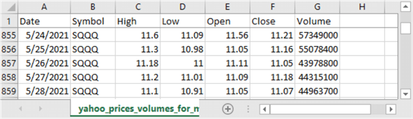
• The image for the second row in the following table shows values for the last five data rows for the SQQQ ticker symbol (again preceded by a row of column headers).
  • The data runs through May 28, 2021, which matches the end date for the downloaded data for the ticker symbol in the preceding Python script (see the code to the left of the third bullet).
  • The row number for the last data row for the SQQQ symbol is 859. Because the first row of data for the SQQQ symbol is row 2, this means that there are 858 rows of data per symbol – one for each trading date from the start date through the end dates.
• The image for the third row in the following table shows the last five rows in the downloaded data.
  • These five rows are for the SDOW ticker symbol which is for the last ticker symbol in the file of six ticker symbols.
  • Notice that the last row number for the SDOW symbol is 5149.
    • Because there is just one row of column headers in the downloaded file, this means that there are 5148 time series data rows in the overall file.
    • This count for the total data rows results from there being 858 rows per symbol and six distinct symbols (6 * 858 = 5148).

Reading the .csv file from Python into SQL Server

The following T-SQL script illustrates one way of importing into SQL Server the .csv file created by Python script in the preceding section.

• The script starts by declaring DataScience as the default database. You can use any other database that is convenient for you on a SQL Server instance.
• Next, the script creates a fresh empty copy of the tickers_jan_2018_may_2021 table. This table is for storing the contents of the .csv file created by the preceding Python script.
• A bulk insert statement populates the tickers_jan_2018_may_2021 table from the .csv file. The statement starts inserting data rows from the second row of the .csv file because the first row contains column headers.
• An alter table statement followed by an alter column statement ensures the volume column has a bigint data type. Yahoo Finance sometimes stores volume values in a real data type. Valid volume values include any positive whole number.
• The script concludes with a select statement to display the values in the tickers_jan_2018_may_2021 table.

use DataScience
go
 
-- this code is to create and populate a set of time series in
-- the dbo.tickers_jan_2018_may_2021 table within DataScience database
 
--conditionally create a table
drop table if exists dbo.tickers_jan_2018_may_2021;
 
create table dbo.tickers_jan_2018_may_2021(
date date,
symbol nvarchar(10),
[high] money,
[low] money,
[open] money,
[close] money,
[volume] float
)
 
-- bulk insert into SQL Server from Python .csv file
bulk insert dbo.tickers_jan_2018_may_2021
from 'C:\python_programs_output\yahoo_prices_volumes_for_mssqltips_list_w_up_and_down_etf_index_tickers_to_csv_demo.csv'
with(format='csv',firstrow = 2);
 
-- convert Python volume output from real to bigint
alter table dbo.tickers_jan_2018_may_2021 
alter column volume bigint;
 
-- display all imported values from Python .csv file
select * from dbo.tickers_jan_2018_may_2021

The following table shows the first and last five rows in the results set from a select statement at the end of the preceding script. Notice that the values in the results set match those from the spreadsheet display of the .csv file contents in the prior section.

Computing exponential moving averages for data from the DataScience database

Up until this point, the current tip added time series for six ticker symbols to the DataScience database. The reason for doing this is to compute a set of exponential moving averages for each symbol’s close price time series. Exponential moving averages can smooth random variations in underlying time series values so that data scientists and other analysts can discern trends as well as changes in trends for time series values.

Exponential moving averages used in financial applications typically have period lengths. An exponential moving average with a short period length will respond very quickly to changes in the underlying time series values. On the other hand, exponential moving averages with longer period lengths will be better at showing medium-term and long-term trends.

MSSQLTips.com published an in-depth tip on computing exponential moving averages using T-SQL for seven different period lengths. The tip on computing exponential moving averages relies on another prior tip for creating a data warehouse for storing time series data. The code for computing exponential moving averages resides in a previously created database named for_csv_from_python. The current tip leverages these two prior tips by transferring period indicator values, such as dates, and time series values, such as close prices, from the tickers_jan_2018_may_2021 table in the DataScience database to the for_csv_from_python database.

• Within the for_csv_from_python database are fact and dimension tables from a data warehouse along with a stored procedure named insert_computed_emas for computing seven exponential moving average values for each close value. The exponential moving averages are different by their period length. The period lengths are 3, 8, 10, 20, 30, 50, and 200. Each period in this tip extends over a span of trading dates.
• The insert_computed_emas stored procedure saves the computed exponential moving averages with different period lengths in the date_symbol_close_period_length_ema table of the dbo schema within the for_csv_from_python database.

The following code segment demonstrates how the tip transfers data from the DataScience database to the for_csv_from_python database.

• As its name implies, the datedimension table in the for_csv_from_python database is a date dimension table in a data warehouse. To fulfill this objective, the table has a date column and other columns for categorizing dates, such as dayname, daynumer, monthname, and monthnumber. You can add additional columns based on your data processing requirements.
• A delete statement removes all prior rows from the datedimension table before re-populating the table based on the dates in the tickers_jan_2018_may_2021 table from the DataScience database.
• The yahoo_prices_valid_vols_only table in the for_csv_from_python database is a fact table for price and volume time series data.
• A truncate table statement removes all prior rows from the yahoo_prices_valid_vols_only table before re-populating the table based on price and volume data from the tickers_jan_2018_may_2021 table in the DataScience database.
• The yahoo_prices_valid_vols_only and tickers_jan_2018_may_2021 tables are both designed to store price and volume time series data, but they were created for different applications that are years apart in terms of their creation dates. Consequently, the column order of the different types of prices (open, high, low, close) is not the same across the two tables. Therefore, the order of the columns needs to be reconciled when copying data from one table to the other. The enumeration of column names in the last select statement of the following script accomplishes this goal.

-- populating two tables in the for_csv_from_python database
-- from the DataScience database
 
-- delete all rows from for_csv_from_python.dbo.datedimension
delete from for_csv_from_python.dbo.datedimension
 
-- reset datedimension table based on tickers_jan_2018_may_2021  table
insert into for_csv_from_python.dbo.datedimension
-- date rows in DataScience.dbo.tickers_jan_2018_may_2021 
select 
     date
    ,datename(weekday, date) dayname
    ,datepart(weekday,date) daynumber
    ,datename(month, date) monthname
    ,datepart(month, date) monthnumber
    ,year(date) year
from DataScience.dbo.tickers_jan_2018_may_2021
where symbol = 'SQQQ'
 
-- truncate yahoo_prices_valid_vols_only table; this is an obsolete fact table
truncate table for_csv_from_python.dbo.yahoo_prices_valid_vols_only 
 
-- this code populates the fact table based on the current time series data and it
-- rearranges column values from the DataScience.dbo.tickers_jan_2018_may_2021 table
-- according to the column order in the for_csv_from_python.dbo.yahoo_prices_valid_vols_only 
insert into for_csv_from_python.dbo.yahoo_prices_valid_vols_only
select date, symbol, [open], high, low, [close], [volume] 
from DataScience.dbo.tickers_jan_2018_may_2021

The next code segment starts by truncating the date_symbol_close_period_length_ema table. This table is used by this tip’s application to store exponential moving averages with different period lengths. The insert_computed_emas stored procedure successively adds new rows in a relational database format to the date_symbol_close_period_length_ema table. Each invocation of the stored procedure passes a parameter for one of the distinct tickers in the yahoo_prices_valid_vols_only table. Within this tip, there are six invocations of the stored procedure – one for each distinct symbol. At the end of these invocations, the date_symbol_close_period_length_ema table has 36,036 rows – one row for each of the seven period lengths times the 5148 rows of time series data across the six symbols.

-- truncate relational table of emas
truncate table [for_csv_from_python].[dbo].[date_symbol_close_period_length_ema]
 
-- run stored proc to save computed emas
exec for_csv_from_python.dbo.insert_computed_emas'UDOW'
exec for_csv_from_python.dbo.insert_computed_emas'SPXL'
exec for_csv_from_python.dbo.insert_computed_emas'TQQQ'
exec for_csv_from_python.dbo.insert_computed_emas'SDOW'
exec for_csv_from_python.dbo.insert_computed_emas'SPXS'
exec for_csv_from_python.dbo.insert_computed_emas'SQQQ'

The following screen shot includes a short T-SQL script for displaying the rows in the date_symbol_close_period_length_ema table. The script sorts the rows by date, symbol, and period length for the computed ema values in the table. The Results pane size is set to show the first 21 rows of the results set for the script in the code window.

• The first seven rows have null ema values.
  • All seven rows are for the first trading date in 2018. There is one row for each of the seven period lengths (3, 8, 10, 20, 30, 50, 200).
  • The ema values for these rows are null because an ema is computed based on the weighted average of the ema from the preceding row and the underlying time series value from the current row.
  • Therefore, the computed ema for the first trading date is null because there can be no preceding ema value for the first ema value.
• The second seven rows all have the same ema column value.
  • All seven rows are for the second trading date in 2018.
  • This is, again, a definitional matter because the ema for the second date is specified by an arbitrary convention. The arbitrary convention used in this tip is that the preceding ema is equal to the underlying time series value for the first period, which is 309.06.
• The third set of seven rows have different ema column values.
  • These ema values are all for the third trading date.
  • Furthermore, the values are different for each row because the weight for the current period’s time series value is different for each row, which is for a different period length.
  • The weight for the preceding period’s ema value also depends on the period length. This weight is also different for each of the seven rows in the third set of seven rows.

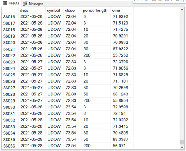
The following screen shot displays the last 21 rows in the date_symbol_close_period_length_ema table.

• These 21 rows are for just three dates:
  • seven for the last trading date in May, 2021;
  • seven more for the next-to-last trading date in May, 2021;
  • and seven more for trading date preceding the next-to-last trading date in May, 2021.

• The first seven rows in the following screen shot are all for the trading date on 2021-05-26. There are seven rows in the set because each trading date has seven ema values – one for each of the period lengths.
• The second set of seven rows are all for the trading date on 2021-05-27.
  • Each of the ema values in the second set of seven rows are larger for corresponding period lengths than ema values in the first set of seven rows.
  • This is because the underlying time series value, the close column value, for the second trading date (72.83) is larger than for the first trading date (72.04).
• The last set of seven rows are all for the trading date on 2021-05-28.
  • The ema values for these seven rows are larger for ema values with matching period lengths than either of the prior two sets of seven rows.
  • This is because the close column value is larger for the last set of seven rows than either of the two preceding sets of seven rows.

Displaying the computed ema values in a non-relational format

The date_symbol_close_period_length_ema table in the previous section stores seven different ema values for each of 5,148 time series values, whose values are unique from each other by symbol and date. The seven different ema values per time series value are derived from seven distinct period lengths so that the whole table contains 36,036 rows – that is, 5148 time series rows times 7 period length rows. While this kind of table design is convenient for joining the ema values to symbols and dates, it leads to a fact table that has many rows.

This section presents another way for storing and displaying ema values for time series data. Instead of storing each ema value with a different period length on a separate row, you can pivot the ema values so that ema values with different period lengths appear in separate columns. By storing ema values with different period lengths in different columns, the number of rows in the table is reduced dramatically, and some business analysts may find the data easier to read. This section demonstrates how to design T-SQL to display the data this way.

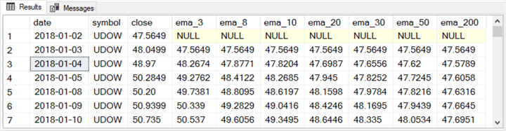
The following table displays the first and last seven rows of a table storing ema values with different period lengths in separate columns instead of separate rows.

• There are just 858 rows in the table.
• Each row is for a distinct date -- starting at the first trading date in 2018 and running through the last trading date in May of 2021.
• All the rows contain close prices and ema values for the UDOW symbol. However, a T-SQL script can easily make it possible to show values for any symbol by assigning a symbol value to a local variable.

Here’s a code segment for creating and populating a table like the one excerpted in the preceding table.

• The @symbol local variable has the string value ‘UDOW’ assigned to it in a declare statement at the top of the script. You can use any of the other five symbols for which data are available.
• An outer query contains seven nested queries named symbol_3, symbol_8, symbol_10, symbol_20, symbol_30, symbol_50, and symbol_200.
• The results set for each of the six remaining queries after the results set for symbol_3 are inner joined to the one for the symbol_3 query. The joins are by date and symbol column values.
  • All the columns from the symbol_3 nested query are referenced in the outer query.
  • Only the column with ema values are referenced in the outer query. For example,
    • This is the ema_8 from the symbol_8 nested query and
    • The column name from the symbol_200 nested query is ema_200

-- display ema values for set of period lengths for UDOW symbol and date
 
declare @symbol nvarchar(10) = 'UDOW'
 
select 
 symbol_3.*
,symbol_8.ema_8
,symbol_10.ema_10
,symbol_20.ema_20
,symbol_30.ema_30
,symbol_50.ema_50
,symbol_200.ema_200
from
(
   select date, symbol, [close], ema ema_3
   from for_csv_from_python.[dbo].[date_symbol_close_period_length_ema] 
   where symbol = @symbol and [period length] = 3
) symbol_3
 
inner join
 
(
   select date, symbol, [close], ema ema_8
   from for_csv_from_python.[dbo].[date_symbol_close_period_length_ema] 
   where symbol = @symbol and [period length] = 8
) symbol_8
 
on symbol_3.DATE = symbol_8.DATE and symbol_3.symbol = symbol_8.symbol
 
inner join
 
(
   select date, symbol, [close], ema ema_10
   from for_csv_from_python.[dbo].[date_symbol_close_period_length_ema] 
   where symbol = @symbol and [period length] = 10
) symbol_10
 
on symbol_3.DATE = symbol_10.DATE and symbol_3.symbol = symbol_10.symbol
 
inner join
 
(
   select date, symbol, [close], ema ema_20
   from for_csv_from_python.[dbo].[date_symbol_close_period_length_ema] 
   where symbol = @symbol and [period length] = 20
) symbol_20
 
on symbol_3.DATE = symbol_20.DATE and symbol_3.symbol = symbol_20.symbol
 
inner join
 
(
   select date, symbol, [close], ema ema_30
   from for_csv_from_python.[dbo].[date_symbol_close_period_length_ema] 
   where symbol = @symbol and [period length] = 30
) symbol_30
 
on symbol_3.DATE = symbol_30.DATE and symbol_3.symbol = symbol_30.symbol
 
inner join
 
(
   select date, symbol, [close], ema ema_50
   from for_csv_from_python.[dbo].[date_symbol_close_period_length_ema] 
   where symbol = @symbol and [period length] = 50
) symbol_50
 
on symbol_3.DATE = symbol_50.DATE and symbol_3.symbol = symbol_50.symbol
 
inner join
 
(
   select date, symbol, [close], ema ema_200
   from for_csv_from_python.[dbo].[date_symbol_close_period_length_ema] 
   where symbol = @symbol and [period length] = 200
) symbol_200
 
on symbol_3.DATE = symbol_200.DATE and symbol_3.symbol = symbol_200.symbol

Instead of demonstrating how to modify the above script for each of six symbols and saving the results sets from the altered scripts in a table, the download for this tip contains two create statements – one for a fresh table, and the other for a fresh stored procedure.

• The code in the download file creates a fresh version of the ema_values_for_period_lengths_by_symbol_and_date table. This table stores the results set from running a stored procedure that returns a results set like the one excerpted in the preceding table.
• The stored procedure is named usp_retrieve_ema_values_for_period_lengths_by_symbol_and_date. The stored procedure accepts an input parameter as a string value with a nvarchar(10) data type.

After running the code to create fresh versions of the table in the DataScience database or whatever other database you use as your default database for running the code in this tip, you can run the following code segment to populate the table for each of the six symbols used in the tip.

• Each insert into statement followed by an exec statement populates the ema_values_for_period_lengths_by_symbol_and_date table for one symbol.
• The select statement at the end of the script displays the ema_values_for_period_lengths_by_symbol_and_date table with the results sets for all six symbols ordered by symbol and date.

-- display ema values by symbol and date
-- run from the default database for the code in this tip
 
insert into dbo.ema_values_for_period_lengths_by_symbol_and_date
exec dbo.usp_retrieve_ema_values_for_period_lengths_by_symbol_and_date 'UDOW'
 
insert into dbo.ema_values_for_period_lengths_by_symbol_and_date
exec dbo.usp_retrieve_ema_values_for_period_lengths_by_symbol_and_date 'SPXL'
 
insert into dbo.ema_values_for_period_lengths_by_symbol_and_date
exec dbo.usp_retrieve_ema_values_for_period_lengths_by_symbol_and_date 'TQQQ'
 
insert into dbo.ema_values_for_period_lengths_by_symbol_and_date
exec dbo.usp_retrieve_ema_values_for_period_lengths_by_symbol_and_date 'SDOW'
 
insert into dbo.ema_values_for_period_lengths_by_symbol_and_date
exec dbo.usp_retrieve_ema_values_for_period_lengths_by_symbol_and_date 'SPXS'
 
insert into dbo.ema_values_for_period_lengths_by_symbol_and_date
exec dbo.usp_retrieve_ema_values_for_period_lengths_by_symbol_and_date 'SQQQ'
 
select * from dbo.ema_values_for_period_lengths_by_symbol_and_date order by symbol, date

The following table contains three excerpts from the results set for the select statement at the end of the preceding code segment.

• The screen shot in the first row in the following table excerpts the first seven rows in the results set.
  • All seven rows are for the SDOW symbol. This is the symbol referenced by the first exec statement in the preceding script.
  • The ema values for row 1 are all null. Recall that ema values do not exist for the first period in a time series.
  • The ema values for row 2 all equal the close value for row 1. This, again, follows from the definition used for an exponential moving average used in this tip.
  • The ema values for rows 3 through 7 are generally distinct because of the expression used to compute exponential moving averages.
• The screen shot showing in the second row in the following table excerpts the last seven rows with ema values for the SDOW symbol. Notice especially that the last row number for the SDOW symbol is 858; this is because there are 858 distinct dates for each symbol.
• The screen shot in the third row of the following table excerpts the last seven rows in the ema_values_for_period_lengths_by_symbol_and_date table.
  • All these rows are for the UDOW symbol, which is the last of the six symbols in alphabetical order. This sort order is from the order by clause at the end of the preceding script.
  • The last row number in the third row from the following table is 5148. This is a valid number of rows considering that the results set is for six sets of 858 rows that total to 5148 rows, which are the number of time series values across all six symbols.

Next Steps

This tip’s download file contains three files to help you get a hands-on feel for building a Python/SQL Server multi-step solution.

1. There is one Python script file with a .py extension. You can use this file to download price and volume data from Yahoo Finance and export the downloaded data in a .csv file.
2. There is a .txt file with the six ticker symbols used in this tip.
3. There is a .sql file with T-SQL scripts demonstrated in this tip. These scripts
   • import the .csv file exported by Python to a SQL Server table
   • compute exponential moving averages for the imported time series data
   • format the computed exponential moving averages as a SQL Server table suitable for import to Python for charting and modeling.

If you ever work with time series data, such as production for manufacturing plants, or weather for a collection of weather stations, or stock symbols, this tip (along with selected prior tips) can reduce your development effort to compute exponential moving averages. Furthermore, upcoming tips will demonstrate charting and modeling techniques for this kind of data.

About the author

Rick Dobson is an author and an individual trader. He is also a SQL Server professional with decades of T-SQL experience that includes authoring books, running a national seminar practice, working for businesses on finance and healthcare development projects, and serving as a regular contributor to MSSQLTips.com. He has been growing his Python skills for more than the past half decade -- especially for data visualization and ETL tasks with JSON and CSV files. His most recent professional passions include financial time series data and analyses, AI models, and statistics. He believes the proper application of these skills can help traders and investors to make more profitable decisions.

This author pledges the content of this article is based on professional experience and not AI generated.

View all my tips