Problem
When I’m reading blog posts or watching videos about how to build a Power BI model, I often hear that the “star schema” is the best way to structure data for aggregation, data integrity, query performance, etc. I’m not familiar with this concept. What does this mean?
Solution
A star schema is a database modeling technique commonly used in data warehousing and business intelligence projects. It is a schema design used to organize and store data in a way that simplifies query processing and reporting in a relational data model. Its basic form consists of a single fact table surrounded by multiple dimension tables, all connected by joins between the primary key and foreign keys (often called surrogate keys).
For example, we can have a fact table tracking Sales data, along with a couple of dimensions that hold descriptive data, such as employee, product, and store:

The “star schema” gets its name from the shape the data model makes when you put the fact table in the center and the dimensions around it, like in the picture above. Another name for the modeling technique is dimensional modeling. It has been around for decades and has been popularized by Ralph Kimball in his book, The Data Warehouse Toolkit: The Definitive Guide to Dimensional Modeling (now in its 3rd edition).
Keep in mind that a star schema can actually have more than one fact table. This is sometimes referred to as a star constellation, but most people use star schema, dimensional model, or data mart. The different fact tables are linked by shared dimensions called conformed dimensions.
Advantages of the Star Schema
The star schema is known for its simplicity, as it requires fewer joins compared to other database models. This makes it easier for users to create queries that are both quick and accurate.
In transactional databases – usually referred to as OLTP systems – data is often normalized. This means the data is structured to avoid redundancy, and consistency is easier to guarantee. There are different normal forms, depending on how far you want to go in the normalization process. Frequently, the 3rd normal form is used.
Using the same example as before, a normalized data model might look like this:

In such a schema, the model is optimized to do as few writes as possible when a change happens. However, when you run large analytical queries on top of this model, you’ll need more joins between the different tables to get the desired result, which slows down performance. With denormalized data in fewer tables, we eliminate many of these joins to improve read performance. Since there’s more redundancy, writes are typically going to be slower. But in an analytical system such as a data warehouse, this isn’t a big problem as data is loaded in batches (usually one or more times a day). In contrast, in an OLTP system, data is continuously changed.
The concepts of facts and dimensions also feel natural to the typical user, as they map neatly to the business domains they use daily. For example, in a typical Excel pivot table, the data from dimensions are used in filters, slicers, or on the axis, while the measures from a fact table are inside the table:

The Importance of Star Schema in Power BI
Because of the way the internal mechanics of a Power BI model work, a star schema is recommended for its data model. It has many performance advantages over other models (especially the model where everything is kept as one giant table). It also simplifies formulas written in DAX (the modeling language of Power BI). The tip, The Importance of a Good Data Model in Power BI Desktop, dives deeper into this topic.
Building Blocks of the Star Schema
In this tip, we mentioned the concepts of dimensions and fact tables several times. In the following paragraph, a short introduction is given. It’s by no means complete, as you’d need an entire book or a complete course to go over all its topics.
Facts
Facts are the numerical measurements of a business process. Some examples of facts are sales, cost of goods, profit and revenue, market share, number of items returned, temperature measured, and so on. They can be quantitative or qualitative and are used to measure a business process. In the AdventureWorks sample data warehouse, we have a couple of example fact tables:

There are two types of facts: additive facts and semi-additive facts. Additive facts are facts that can be added up over any dimension. For example, sales revenue is an additive fact because it can be added over any dimension, such as customer, product, or time. Semi-additive facts can be added up over some dimensions, but not all. For example, inventory can be added up over product and warehouse, but not over time. For example, if you had 15 crates of bananas yesterday and 12 crates today (meaning you sold 3 crates), you cannot sum these up and report that you had 27 crates over two days. You can argue that there are also non-additive facts, such as the temperature measured in weather stations. These cannot be added up over any dimension.
There are three types of fact tables (which can all contain additive and/or semi-additive facts):
- Transactional. These fact tables record the different transactions of a business process. Sales is a good example, but also the actual transactions of a bank account. Transactional fact tables are the most common.
- Snapshot. In this fact table, a snapshot of the data is loaded into the table every day. This can be the inventory of a shop but also the balance of your bank account. These fact tables are typically very large (one million bank accounts means one million rows are added daily. They also contain semi-additive measures, where you can usually not add the measure up over time. It wouldn’t make sense to take a sum of your account balance over the different days.
- Accumulating Snapshot. This fact table models a process with a well-defined lifecycle. For example, the returns process of an item, claims processing in an insurance company, college admissions, and sales funnels. These fact tables have a lot of date columns, where each date marks a specific step in the lifecycle. As opposed to the other types of fact tables, this table is updated often; each time a record progresses through the cycle, a specific date is updated.
Fact tables are typically very long, contain many rows, and have a lot of numeric columns (the actual facts themselves, but also the foreign keys to all the dimensions). String columns (or other long data types) are to be avoided to improve performance.
Dimensions
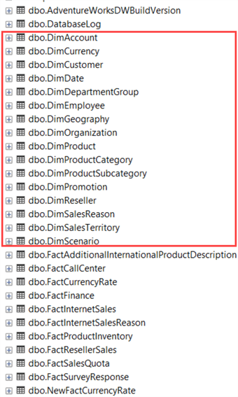
Dimensions contain the descriptions of a fact. They provide context, granularity and add meaning to a fact. Customer, product, time, employee, or geography are examples of dimensions. In contrast to fact tables, they don’t contain many rows but typically have many columns. Every attribute the end-user wants to filter on, slice on, or put on the axis of a visual or matrix in Power BI comes from a dimension. Since business users want to view a problem from all different angles, many attributes are needed. It’s not uncommon to have more than 50 columns in a dimension. In the Adventure Works database, we can find the following dimensions:
Dimensions can also track history. If a record is updated in the source system, a dimension in the DWH can hold both the old and the new value, which can be very useful in reporting and analytics. When history is tracked, we speak of slowly changing dimensions (SCD).
There are three types of SCDs:
- Type 1: This type of SCD is used to overwrite any data changes that occur over time. When an existing record is modified, the new values replace the old ones completely. This type doesn’t track history.
- Type 2: This type of SCD tracks changes over time by creating new versions of a record. A new version is inserted with the new data when a value is changed, while the old version is still retained and can be referred to at any time.
- Type 3: This type of SCD tracks changes over time and creates multiple versions of the same record. The latest versions of the record will always be visible, and some or all previous versions are stored as well. This type isn’t often used but can be useful, for example, after a data migration. Let’s illustrate with an example where we track the previous e-mail of a customer. When an e-mail changes, we add a column that will keep the old value while the original column holds the new value.

There are more types of slowly changing dimensions (usually a combination of the three first types). If you’re interested in more detail, check out the Kimball book.
Next Steps
- Another great resource to learn more about star schema modeling is the book Star Schema – The Complete Reference.
- To learn more about how to implement slowly changing dimensions of type 2, check out the following tips:
- How to Create a Star Schema in Power BI Desktop
- Create a Star Schema Data Model in SQL Server using the Microsoft Toolset
- Explore the Role of Normal Forms in Dimensional Modeling

Koen Verbeeck is a seasoned business intelligence consultant with over a decade of experience with the Microsoft Data Platform. He holds several certifications, including Azure Data Engineer. He’s a prolific writer, with over 375 articles on technologies such as Microsoft Fabric, SSIS, ADF, SSAS, SSRS, MDS, Power BI, Snowflake and Azure services. He has spoken at various events such as PASS, SQLBits, dataMinds Connect and many others. He frequently delivers educational webinars on MSSQLTips.com. For his efforts, Koen has been awarded the Microsoft MVP data platform award for many years.
- MSSQLTips Awards:
- Leadership Award (200+ Tips) – 2021
- Author of the Year – 2014/2020/2022
- Author Contender – 2024/2025