Three Use Case Examples for SQL Subqueries

By: Rick Dobson   |   Updated: 2023-03-22   |   Comments   |   Related: > TSQL

Problem

There are many great tutorials on syntax, performance, and keywords for invoking subqueries. However, I wish to discover a tip highlighting selected SQL subquery use cases. Please briefly describe three SQL subquery use case examples. For each use case, cover how a subquery interacts with outer queries and the T-SQL for implementing the use case. Review excerpts from each example to show the value of implementing the use case.

Solution

For readers who want help with subquery syntax, performance, or keyword issues, you may find what you need in one of these prior tips from MSSQLTips.com:

• Introduction to Subqueries in SQL Server
• SQL Server Uncorrelated and Correlated Subquery
• SQL Server Subquery Example
• SQL Server Derived Table Example
• SQL Server IN vs EXISTS
• SQL NOT IN Operator

Additionally, a few minutes of internet searching will return many more tips about subqueries in MSSQLTips.com and other sources.

After you learn the basics of what subqueries are, you may like to review some examples that illustrate how to apply subqueries for typical SQL developer tasks. This tutorial provides three use case examples with SQL code and illustrative result set excerpts for each use case to help you rapidly understand each example. The presentation of use case examples includes a link to a prior tip with the source data for the example to help you to re-run the examples in the tip.

Quick Highlights about Subquery Design Issues

A subquery is a query that resides in and returns values to an outer query. The subquery typically returns a scalar value, a column of values, or a multi-row, multi-column results set. The return results set can be fixed by hard-coding parameters for the subquery and not modifying referenced data source, or the results set can be dynamic by conditioning subqueries on local variables and referencing external data sources that are updated regularly. Combining an outer query and its subquery typically provides a results set for display, data visualization in various chart formats, or populating a data warehouse.

You can insert a subquery in the select list, from clause, or the where clause of an outer query. Subquery examples with each of these use cases are illustrated in this tip.

Use Case #1: Segmenting the Rows of a Table

The first subquery use case is to segment some source data into two segments; this is a classic subquery use case. The use case's implementation in this section is representative of cases where data are received daily, weekly, or monthly from multiple providers for populating a data source and generating reports.

This use case example draws on data from the yahoo_finance_ohlcv_values_with_symbol table. The steps for downloading CSV files from Yahoo Finance to a SQL Server table are described in this prior tip (A Framework for Comparing Time Series Data from Yahoo Finance and Stooq.com). The download in the prior tip includes 62 CSV files downloaded from Yahoo Finance that populate the yahoo_finance_ohlcv_values_with_symbol table; there is one file for each ticker symbol. The prior tip also shows the steps to transfer the files to the SQL Server table.

Here are two queries for the data in the use case for this section.

• The first query counts the number of rows in the yahoo_finance_ohlcv_values_with_symbol table. This query serves as the outer query for the use case in this section.
• The second query computes the average close column value in the yahoo_finance_ohlcv_values_with_symbol table. The following query serves as the subquery for the use case example.

-- count of rows in yahoo_finance_ohlcv_values_with_symbol
-- there are 284411 rows in the source data table
select count(*) [row count in yahoo_finance_ohlcv_values_with_symbol]
from [DataScience].[dbo].[yahoo_finance_ohlcv_values_with_symbol]
 
-- avg close value across all symbol and date values
-- the average close column value is 4336.9954
select avg([close]) [avg close value across all rows in yahoo_finance_ohlcv_values_with_symbol] 
from [DataScience].[dbo].[yahoo_finance_ohlcv_values_with_symbol]

The following SQL statement lists the data in yahoo_finance_ohlcv_values_with_symbol by symbol and date.

select [symbol]
      ,[date]
      ,[open]
      ,[high]
      ,[low]
      ,[close]
      ,[volume]
from [DataScience].[dbo].[yahoo_finance_ohlcv_values_with_symbol]
order by symbol, date

The following two screenshots show excerpts from the results set from the preceding script, with the first five and last five rows ordered by ticker symbol and date. The first column with row numbers in the second screenshot shows 284411 rows in the table. By changing the source table, you can readily apply the example to other kinds of data, such as sales, production, equipment tracking, etc.

Here are two examples that show the syntax for inserting the query that computes average close column values as a subquery within the outer query for counting the number of rows in a results set. In each example, the subquery appears in the where clause of the outer query.

• The first query counts the number of rows whose close column values are greater than the average close column value.
• The second query counts the number of rows whose close column values are less than or equal to the average close column value.
• The counts returned by each subquery example are in the comments before each subquery example.

-- count for rows with above average close
-- there are 11547 rows with close values above the average close value
select count(*) [count for rows with above average close]
from [DataScience].[dbo].[yahoo_finance_ohlcv_values_with_symbol]
where [close] >
(select avg([close])
from [DataScience].[dbo].[yahoo_finance_ohlcv_values_with_symbol])
 
-- count for rows with close values less than or equal to average close
-- there are 272864 rows with close values less than or equal to the average close value
select count(*) [count for rows with close values less than or equal to average close]
from [DataScience].[dbo].[yahoo_finance_ohlcv_values_with_symbol]
where [close] <=
(select avg([close])
from [DataScience].[dbo].[yahoo_finance_ohlcv_values_with_symbol])

The final query for this use case example is next. It verifies the row counts from each of the preceding subquery examples. The query confirms that the sum of row counts from each use case example equals the total number of rows in the yahoo_finance_ohlcv_values_with_symbol table.

-- SQL to verify row counts for above average and at or below average rowsets
-- select (11547 + 272864) = 284411
select 
 
(
select count(*) [count for rows with above average close]
from [DataScience].[dbo].[yahoo_finance_ohlcv_values_with_symbol]
where [close] >
(select avg([close])
from [DataScience].[dbo].[yahoo_finance_ohlcv_values_with_symbol])
)
 
+ 
 
(
select count(*) [count for rows with close values less than or equal to average close]
from [DataScience].[dbo].[yahoo_finance_ohlcv_values_with_symbol]
where [close] <=
(select avg([close])
from [DataScience].[dbo].[yahoo_finance_ohlcv_values_with_symbol])
) [verified sum of row counts]

Use Case #2: Joining Derived Table Columns from a Subquery to an Outer Query's Results Set

A derived table is a results set based on a T-SQL query statement that returns a multi-row, multi-column results set based on one or more underlying data sources. After specifying a derived table, you can join it with the results set from an outer query. Then, you can incorporate references for a subset of derived table columns in the select list for the outer query.

Another way to populate column values for select list items in an outer query from a subquery is with an embedded or nested SELECT statement. Avoid this approach whenever possible because it can result in row-by-row operations. While embedded select statements may be a fast way for some analysts to express a relationship, query performance on large to intermediate-sized datasets is much faster for converting embedded select clauses to a derived table that is joined to a table in an outer query.

• The embedded select statement must return a scalar value.
• The scalar value returned by the embedded select statement populates a single column value for each row in the results set from the outer query.
• The subquery use case example in this section illustrates subquery examples based on joined derived tables and embedded select statements.

Here is the code for the use case example in this section. A derived table subquery is joined to a table from an outer query:

• The select statement for the outer query references the yahoo_finance_ohlcv_values_with_symbol table in its from clause; the data source in the from clause has an alias of outer_query.
• After the join keyword trailing the select statement for the outer query in the use case example, a subquery named sub_query_for_first_and_last_closes appears. This subquery is for a derived table.
  • The derived table references the yahoo_finance_ohlcv_values_with_symbol in its from clause.
  • The first column is for the symbol column from the source data table. A group by clause after from clause groups its results set by symbol.
  • The second column in the select statement is named first _date; this column is from the min function of the date column in the derived table.
  • The third column in the select statement is named last_date; this column is from the max function of the date column in the derived table.

There are three pairs of columns in the select list for the outer query:

• The first pair in the select list displays two columns named symbol and date from the data source named outer_query.
• The second pair of items in the select list illustrates the syntax for specifying the inclusion of the first_date and last_date columns from the derived table.
• The third pair of items is based on two nested select statements
  • Each of the select statements references the yahoo_finance_ohlcv_values_with_symbol table in their from clause
  • The where clause in each select statement matches the embedded query to the outer query on a row-by-row basis
    • the symbol column from the outer query to the symbol column from the derived table (sub_query_for_first_and_last_closes) and
    • the date column from the outer query to the date from the derived table
    • it is the row-by-row matching that makes nested select statements a less preferable option from a performance perspective than a join to a subquery from the outer query
  • The first nested select statement returns a column of values named first_date_close
  • The second nested select statement returns a column of values named last_date_close

-- close values by symbol by date in ASC order
select
 outer_query.symbol
,outer_query.date
,sub_query_for_first_and_last_closes.first_date
,sub_query_for_first_and_last_closes.last_date
,(select [close] from [DataScience].[dbo].[yahoo_finance_ohlcv_values_with_symbol] 
  where sub_query_for_first_and_last_closes.symbol = symbol and sub_query_for_first_and_last_closes.first_date = date) first_date_close
,(select [close] from [DataScience].[dbo].[yahoo_finance_ohlcv_values_with_symbol] 
  where sub_query_for_first_and_last_closes.symbol = symbol and sub_query_for_first_and_last_closes.last_date = date) last_date_close
from [DataScience].[dbo].[yahoo_finance_ohlcv_values_with_symbol] outer_query
 
join
 
(
-- first and last date by symbol
select 
 symbol
,min(date) [first_date]
,max(date) [last_date]
from [DataScience].[dbo].[yahoo_finance_ohlcv_values_with_symbol]
group by symbol
) sub_query_for_first_and_last_closes
 
on outer_query.symbol = sub_query_for_first_and_last_closes.symbol
and outer_query.date = sub_query_for_first_and_last_closes.first_date
 
order by outer_query.symbol

Here are the first 10 of 62 rows from the results set from the preceding query; there is one row for each ticker symbol. Most of the ticker symbols have a first_date column value of 2000-01-03, but one ticker symbol (BOIL) in the display has a first_date column value of 2011-10-07, which is its initial public offering date. There are additional tickers in the full set of 62 rows with initial public offering dates after 2000-01-03.

It is often useful in business applications to document unit tests for a solution. The following code is an example of unit test code for the subquery example in the preceding screenshot for three symbols (AAPL, BOIL, BRK-B). The code uses the top keyword followed by a value of 1 and an order by clause with a keyword of ASC or DESC, respectively, to specify an ascending or descending order.

• The ascending order returns the first_date value for a ticker symbol
• The descending order returns the last_date value for a ticker symbol

-- selected queries for unit tests
select top 1
 symbol
,date
,[close]
from [DataScience].[dbo].[yahoo_finance_ohlcv_values_with_symbol]
where symbol = 'AAPL'
order by date ASC
 
select top 1
 symbol
,date
,[close] 
from [DataScience].[dbo].[yahoo_finance_ohlcv_values_with_symbol]
where symbol = 'AAPL'
order by date DESC
 
select top 1
 symbol
,date
,[close]
from [DataScience].[dbo].[yahoo_finance_ohlcv_values_with_symbol]
where symbol = 'BOIL'
order by date ASC
 
select top 1
 symbol
,date
,[close] 
from [DataScience].[dbo].[yahoo_finance_ohlcv_values_with_symbol]
where symbol = 'BOIL'
order by date DESC
 
select top 1
 symbol
,date
,[close]
from [DataScience].[dbo].[yahoo_finance_ohlcv_values_with_symbol]
where symbol = 'BRK-B'
order by date ASC
 
select top 1
 symbol
,date
,[close] 
from [DataScience].[dbo].[yahoo_finance_ohlcv_values_with_symbol]
where symbol = 'BRK-B'
order by date DESC

Here is the results set from the preceding script:

• Both AAPL and BRB-K have a first date value of 2001-01-03.
• However, BOIL has a first date value of 2011-10-07.

The results set from the very basic lookup code from the unit test verify the results set from the more advanced code in this section's subquery example.

Use Case #3: Computing Seasonality Factors by Month Across Year

There are multiple ways to assess seasonality in time series data. This tip implements a technique presented in an article from StockCharts.com. This section focuses on using a SQL Server subquery to code a solution presented and discussed in StockCharts.com. If you have another favorite method for computing seasonality, consider adapting the coding solution covered here to your favorite method.

Additionally, this section uses a different historical data source for the securities price and volume data. The data source was introduced in a prior MSSQLTips.com article, which includes CSV files downloaded from Yahoo Finance and code for importing the CSV file contents into a table named symbol_date. This tip references the symbol_date table from the DataScience database.

The inner-most query in the solution appears as a stand-alone query in the following script.

• The script starts with a declare statement for the @symbol local variable; the declare statement assigns a value of ‘SPY' to the @symbol variable.
• The following select statement pulls symbol, date, and close column values from the symbol_date table.
• Additionally, the year, month, and a datename function extract, respectively, the year, month number, and month abbreviation from the date value for the current row.
• The select statement's where clause restricts the results set to rows with a value to the current value of @symbol, which is SPY in this section; there are rows for five other ticker symbols in the symbol_date table.

-- pull source data for computing monthly cyclical factors
declare @symbol nvarchar(10) = 'SPY'
 
-- innermost query
-- daily close values for @symbol ticker during year and month
select
 symbol
,date
,year(date) year
,month(date) month
,cast(datename(month, date) as nchar(3)) month_abr
,[close] [close]
from DataScience.dbo.symbol_date
where Symbol = @symbol

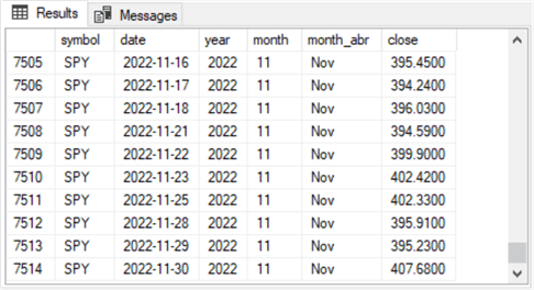
Here are two screenshots from the results set from the preceding script showing the first and the last 10 rows.

• The first screenshot starts with a row having a date value of 1993-02-01.
• The second screenshot ends with a row having a date value of 2022-11-30.

The next code block starts with a go keyword. This terminates the batch in the preceding script window from the batch for the following script window. The script file for computing seasonality actually contains three SQL Server batches. The last batch is displayed and described at the end of this tip section.

• After the go keyword, a declare statement reinitializes the @symbol local variable. By reinitializing the @symbol local variable, the second batch can run without depending on the declare statement in the preceding script window.
• The select statement in the outer query depends on the nested inner-most query.
  • The inner-most query is the subquery that has a name of for_first_and_last_monthly_closes.
  • The inner-most query resides in the outer query's from clause.
• The columns for the results set from the outer query's select statement are as follows:
  • The symbol, year, month, and month_abbr columns are inherited from the inner-most query.
    • The column names appear with and without a prefix indicating their source.
    • The only time that a prefix is required is when column names for outer and inner queries have the same name; consistently using a prefix for the source can improve the readability of the code, but omitting a prefix when it is not required results in a more compact script file.
  • The first_close and last_close columns depend, respectively, on first_value and last_value window functions.
    • These functions extract the first and last close value by year and month from the subquery's results set.
    • However, the first_value function and the last_value function return a value for each trading date in a month -- not just the first and last trading day in a month.
    • The distinct keyword right after the select keyword removes the duplicate first_close and last_close values so that the select statement displays just one first_close column value and just one last_close column value for each year and month combination.
  • The increase_in_month column is defined by a case statement that:
    • Assigns a value of 1 when the first close value for a month is less than the last close value for a month or
    • 0 otherwise
    • This column is used by the outer-most query in the next script window.
• The order by clause at the end of the code block sorts the rows by month.

declare @symbol nvarchar(10) = 'SPY'
 
-- first-level query 
-- first and last close by year, month for @symbol ticker
select distinct
 symbol
,year
,for_first_and_last_monthly_closes.month
,month_abr
,first_value([close]) OVER (partition by year, month order by month) first_close
,last_value([close]) OVER (partition by year, month order by month) last_close
,
 case
   when first_value([close]) OVER (partition by year, month order by year, month) < 
      last_value([close]) OVER (partition by year, month order by year, month)
      then 1
   else 0
 end increase_in_month
from
(
-- innermost query
-- daily close values for @symbol ticker during year and month
select
 symbol
,date
,year(date) year
, month(date) month
,cast(datename(month, date) as nchar(3)) month_abr
,[close] [close]
from DataScience.dbo.symbol_date
where Symbol = @symbol
) for_first_and_last_monthly_closes
order by for_first_and_last_monthly_closes.month

Here are two excerpts from the results set for the preceding script. The first and the second screenshots display the first and last 40 rows, respectively, in the results set from the preceding script. There are either 30 or 29 rows per month and year for each symbol.

• The first screenshot includes just 29 rows for January. This is because the first month for which data were collected from Yahoo Finance was the first trading day in February 1993.
• All the remaining years have 30 rows each, except for 2022. This is because no data were collected after the last trading day in November 2022. Therefore, there are also just 29 rows for 2022.

The final code block for the SPY ticker symbol appears next. This code block embraces the preceding code block in the same way that the preceding code block embraces the inner-most code block. The purpose of the following script is to compute monthly seasonality factors.

The outer-most query in the following script computes the seasonality factors for each month. The seasonality factors are based on the increase_in_month column values computed in the preceding query.

• The sum of the increase_in_month values for a month is how many times the first close value for a month is less than the final close value for a month.
  • When the final close value in a month exceeds or matches the first close value in a month, this means that the price of a share rose or stayed the same from the beginning of the month relative to the end of the month in a year.
  • When the final close value in a month is less than the first close value in a month, it means that the price of a share fell from the beginning of the month relative to the end of the month in a year.
• The count of the increase_in_month values for a month is the total number of years in which the increase_in_month column value can be 1 or 0. Recall that this count is 29 for January and December but 30 for the remaining months.
• The ratio of the sum of the increase_in_month column values divided by the count of the increase_in_month reflects the percent of times during a month that prices were stable or increasing during a month. The multiplication of the ratio by 100 and the casting of the multiplied value as a dec 5,2 data type reflects the percent of stable or increasing monthly outcomes for a month as a decimal value with two spaces after the decimal point.

-- compute monthly seasonality factors for a ticker
declare @symbol nvarchar(10) = 'SPY'
 
select
 symbol
,month
,sum(increase_in_month) increasing_month_instances
,count(increase_in_month) total_month_instances
,cast(((cast(sum(increase_in_month) as dec(5,2))/(count(increase_in_month)))*100) as dec(5,2)) [monthly percent up]
from
(
-- first-level query 
-- first and last close by year, month for @symbol ticker
select distinct
 symbol
,year
,for_first_and_last_monthly_closes.month
,month_abr
,first_value([close]) OVER (partition by year, month order by month) first_close
,last_value([close]) OVER (partition by year, month order by month) last_close
,
 case
   when first_value([close]) OVER (partition by year, month order by year, month) < 
      last_value([close]) OVER (partition by year, month order by year, month)
      then 1
   else 0
 end increase_in_month
from
(
-- innermost query
-- daily close values for @symbol ticker during year and month
select
 symbol
,date
,year(date) year
, month(date) month
,cast(datename(month, date) as nchar(3)) month_abr
,[close] [close]
from DataScience.dbo.symbol_date
where Symbol = @symbol
) for_first_and_last_monthly_closes
)for_sum_of_increases_and_count_of_year_months
group by symbol,month

Here is the output from the preceding script.

• The SPY is an exchange traded fund based on the S&P 500 index. The approximately 500 stocks in the index include many leading US stocks.
• Therefore, you might expect the seasonality to be greater than or equal to 50 percent for most months, and it is for 11 of 12 months.
  • The only month that prices fail to increase or remain stable more than 50 percent of the time is June.
  • The likelihood of rising or stable prices is at its highest during the last three months of the year (October through December) for the SPY ticker; seasonality can vary somewhat by ticker.
  • These outcomes partially confirm the validity of the aphorism, which states, "sell in May and go away." For the results in this tip for the SPY ticker, it seems the aphorism could be changed to: "sell in May and go away for a month, then buy your SPY shares back."

This solution presented in this section is an interesting use case for subqueries that is relatively easy and fast to implement. It also addresses a typical business requirement – namely, computing seasonality.

Next Steps

Look into ways of incorporating subqueries into your solutions. They introduce flexibility into what you can accomplish. Furthermore, they are also relatively easy to program.

Subsequent tips will explore additional subquery use case examples to reveal more contexts in which subqueries can enhance the power of SQL Server solutions.

About the author

Rick Dobson is an author and an individual trader. He is also a SQL Server professional with decades of T-SQL experience that includes authoring books, running a national seminar practice, working for businesses on finance and healthcare development projects, and serving as a regular contributor to MSSQLTips.com. He has been growing his Python skills for more than the past half decade -- especially for data visualization and ETL tasks with JSON and CSV files. His most recent professional passions include financial time series data and analyses, AI models, and statistics. He believes the proper application of these skills can help traders and investors to make more profitable decisions.

This author pledges the content of this article is based on professional experience and not AI generated.

View all my tips