Assessing with SQL and Data Science Goodness of Fit to Different Distributions

By: Rick Dobson   |   Comments   |   Related: > TSQL

Problem

Please provide a general framework with SQL code based on data science practices for assessing if a set of data values conform to any of several commonly used distribution types.  For example, start with a framework that works for assessing the goodness of fit of data values to uniform, normal, and exponential distributions.  Design the framework so that it can readily accommodate other distribution types as the need to assess goodness of fit for them arises.  Also, structure the solution so that it is like other components in the SQL Statistics Package.

Solution

Data science is sometimes defined as the use of coding, statistics, modeling, and analysis in a data-centric activity.  A common data-centric activity is assessing if data values allow the confirmation or rejection of a hypothesis about some data values.  For example, a casino might be interested in assessing if a series of die rolls by a game player are from a fair die that shows each die face equally often in the long run; this is an example of testing if outcomes are uniformly distributed.  Alternatively, a call center may want to know for scheduling call takers whether the distribution between calls and the average time between the calls to the center is the same for different day parts, such as from 2 AM through the 9 AM hour, from 10 AM through the 5 PM hour, and 6 PM through the 1 AM hour; this kind of issue can be examined by determining if the probability density of the time between calls is exponentially distributed with the same shape for different day parts.  These and many other data-centric questions can be answered by assessing the goodness of fit of data to a variety of different distribution types.

MSSQLTips.com previously addressed how to design SQL scripts for assessing the goodness of fit of a set of data values to uniformly, normally, and exponentially distributed values ( "Assessing with SQL Goodness of Fit to an Exponential Distribution" and for tip titled "Assessing with SQL Goodness of Fit to Normal and Uniform Distributions").  This tip extends that earlier work by presenting an integrated framework for assessing goodness of fit to all three distribution types.  Additionally, code samples are provided illustrating how to generate uniformly, normally, and exponentially distributed sets of values; this capability is useful for testing the new framework and for Monte Carlo simulations more generally.  The framework presented in this tip applies generally to other types of distributions because new modules for other distributions can be readily added to it.  The programmatic interface design presented in this tip can be readily modified to accommodate new modules for distributions not explicitly addressed in this tip.

You can download all of the scripts for this tip at the bottom of this article.

Overview of a Chi Square Goodness-of-fit test

One especially robust way of assessing goodness of fit for the values in a data set to a distribution type is to use the Chi Square goodness-of-fit test.  This test requires that you segment the data values according to a set of bins or categories.  Then, you can compare by bin how the count of observed values conforms to the expected count from a distribution.  The Chi Square goodness-of-fit test is for a null hypothesis of no difference between the observed and expected counts.  If the computed Chi Square value across bins exceeds or equals a critical Chi Square value, then the null hypothesis is rejected, and the sample values do not conform to the distribution type from which the expected values are derived.  On the other hand, if the computed Chi Square value is less than a critical Chi Square value, then the observed counts are not statistically different from the expected counts.  Therefore, the observed counts cannot be assessed as different from the distribution used to derive expected counts.

The pre-processing for a Chi Square goodness-of-fit test maps each sample observation value to a bin.  The Excel Master Series blog denotes bin characteristics for a valid Chi Square test.  These are as follows.

• The number of bins must be greater than or equal to five.
• The smallest expected frequency in any bin must be at least one.
• The average count of expected values across bins must be at least five.

The bin boundaries can be defined based on the observed values.

• When dealing with discrete values, such as the outcome of die rolls, the bins can be defined by the numbers: 1, 2, 3, 4, 5, and 6.  Similarly, if you were testing whether the number of sales were the same on every day of the week, then the bins can be denoted by the name of the days in a week, such as Sunday, Monday, Tuesday, Wednesday, Thursday, Friday, and Saturday.
• When dealing with continuous values, such as the time, distance, or temperature, a solution framework must specify bottom and top values for a set of bins that span the range of values in a data set.
  • From a statistical perspective, you can think of the smallest bottom bin value as -∞ (or zero when negative values are not allowed) and the largest top bin value as +∞.  From a practical computing perspective for any particular sample of values, the smallest bottom bin value can also start at the lowest sample value and the largest top bin value can map to the greatest sample value.
  • The bottom and top bin values for other bins can be arbitrarily defined subject to the three characteristics for a valid Chi Square goodness-of-fit test denoted above.
  • The code in this tip automatically computes bin boundaries.  One interesting topic for future data science research may be to evaluate alternative strategies for the selection of bin boundaries across different distribution types.

After bins are defined, count the observed values in each bin.  Next, calculate the expected frequencies in each bin according to a distribution function, such as a uniform distribution.

Next, use the following expression to compute a Chi Square value for the counts of a set of sample observed values relative to the expected frequencies by bin.  The i values identify specific bins.  The O_i values represent observed counts for bins.  The O_i values depend on how sample observation values are distributed across bins.  The E_i values represent expected counts per bin.  The E_i values depend on the distribution type and the bin boundaries.  For the purposes of this tip, you can think of the ∑ sign as a sum function over i bins.

∑ ((Oi – Ei)2/Ei)

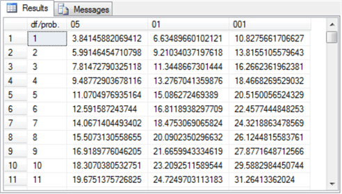
The Excel CHISQ.INV.RT built-in function generates critical Chi Square values for specified degrees of freedom and designated probability levels.  Both of the prior two MSSQLTips.com tips on Chi Square goodness-of-fit tests ("Assessing with SQL Goodness of Fit to an Exponential Distribution" and for tip titled "Assessing with SQL Goodness of Fit to Normal and Uniform Distributions") explain how to use the Excel function and transfer its values to a SQL Server table.  For the Chi Square goodness-of-fit solutions described in this tip, the table must exist in the database from which you are running the SQL code.  The following script specifies the table design for a table named Chi Square Critical Values 05 01 001; this table is to contain critical Chi Square values.

• The df/prob. column holds integer values for the degrees of freedom associated with a computed Chi Square value.
• The 05, 01, and 001 columns store critical Chi Square values, respectively, at the .05, .01, and .001 probability levels.

CREATE TABLE [dbo].[Chi Square Critical Values 05 01 001](
   [df/prob.] [int] NULL,
   [05] [float] NULL,
   [01] [float] NULL,
   [001] [float] NULL
)

The degrees of freedom depend on the number of bins and the type of distribution.  In general, the degrees of freedom value equal the total bins less one to reflect that one bin count is fixed if you know the total number of observed values.  Additionally, reduce this quantity by the number of parameters for the distribution to which you are trying to assess goodness of fit.  The number of parameters for uniform, normal, and exponential distributions are, respectively, zero, two, and one.

The following Results tab displays an excerpt from the Chi Square Critical Values 05 01 001 table.  The excerpt shows the critical Chi Square values for the .05, .01, and .001 probability levels at degrees of freedom one through eleven.  The full set of values in the Chi Square Critical Values 05 01 001 table used in this tip has degrees of freedom for values one through one hundred twenty.

Main purpose of this tip

The main purpose of this tip is to integrate the functionality of three independent SQL scripts – one each for uniform, normal, and exponential distributions -- into one SQL Server application that accommodates three different distributions.  Furthermore, the SQL Server application is designed so that it is relatively easy to add other types of distributions as need arises later.

The transformation from three separate scripts into a single SQL Server application is based on three design principles.

• The goodness-of-fit assessment for any type of distribution starts by reading the values of a data set into a temporary table for subsequent processing.  The data type for values in the temporary table depends on the type of variable you are processing.
  • When working with a discrete variable, such as the number of sales on each day of the week, you can use a varchar data type.
  • When working with a continuous variable, such as the time between calls to a call center, you can use a float data type.
• The subsequent processing depends on:
  • the values in the temporary table
  • the type of distribution
• The framework operates like other components in the SQL Statistics Package.  This tip adds an inferential statistics capability to the SQL Statistical Package.  The inference is about whether a set of counts for observed sample values conform to the expected counts based on a specified distribution.

Code review for SQL Server application

The application described in this tip consists of a pair of stored procedures that are invoked for each type of distribution.  Additionally, there is a script that invokes the stored procedures and configures a global temporary table (##temp) for receiving data.  There is always a single column in the ##temp table, but the column's name and data type vary depending on whether the sample data values are discrete or continuous.  The script calling the stored procedures specifies the column name and data type so that they are appropriate for the goodness-of-fit test to whatever distribution is being assessed.

• The first stored procedure uses the bulk insert command to read data from a txt file.  This stored procedure is the same for all distributions in this tip.  The stored procedure accepts an input parameter specifying the file name and path for the txt file containing the sample data.  While the source file can vary, the destination table (##temp) does not vary.
• The second stored procedure varies by distribution type.  The main purpose of this stored procedure is to assess the goodness of fit for the data in the ##temp table relative to a distribution type.  The details of how to assess goodness of fit vary by distribution type.  The application described in this tip has three versions of this second stored procedure – one for the uniform distribution, another for the normal distribution, and a third for the exponential distribution.

The pairs of stored procedures are invoked from within different batches.  Each batch is for the combination of a distribution type and a sample data set.  Additionally, each pair of stored procedures can run more than once.  For example, if you are assessing two sample data sets for each distribution, then the script will invoke the pair of stored procedures twice – once for each sample data set.  This tip assesses each distribution type for two distinct data sets.

The application needs a way of identifying which type of distribution to test for with each sample data set.  The script designates the type of distribution for which to assess goodness of fit by specifying a row in a temporary table named #crossbatch_variables.  Each row in the temporary table designates one of the three distribution types used in this tip.  However, you can readily add more rows for other types of distributions.  Each distribution type requires its own distinct second stored procedure that performs the goodness of fit for a sample data set after it is read.  The first stored procedure is the same for all distributions, but the framework specifies a different column name and data type for the ##temp table column depending on whether the data set being assessed for goodness of fit includes discrete or continuous variable values.  The code for this tip assumes the uniform distribution is always assessed for a discrete variable, but the normal and exponential distributions are always assessed for a continuous variable.

The remainder of this section reviews the parts of the script that invokes the two stored procedures for:

• the introduction section specifying legitimate distribution types in the #crossbatch_variables temporary table
• the code for invoking the pair of stored procedures for the first data set
• the code for invoking the pair of stored procedures for the second data set

The first data set for each distribution type is based on a previously published sample that was also analyzed in a prior MSSQLTips.com tip.  The first data set for each assessment is chosen because it does not conform to the distribution for which goodness of fit is being assessed.  The second data set for each distribution type is based on a freshly developed sample that is known to conform to one of the three distributions tested for in this tip.  Therefore, the code evaluates each distribution type with one sample that is supposed to fail the goodness-of-fit test and a second sample that is supposed to pass the goodness-of-fit test.

The initial code segment (see the next script excerpt) specifies the legitimate distribution types.  Each legitimate distribution type is designated by a separate row in the #crossbatch_variables temporary table.  By assigning row values for a temporary table different SQL code batches can refer to the temporary table as if its rows contained values for local variables that were global across all batches.

The demonstration in this tip runs inside the AllNasdaqTickerPricesfrom2014into2017 database.  However, you can use any other database you prefer.  Switch use statements to point at any database you prefer to use instead.  Also, be sure the Chi Square Critical Values 05 01 001 table is created and populated in whatever database you choose to use.

The following code block has two operational segments and a third optional segment with a single line of code with a preceding comment marker (--).

• The first segment creates a fresh copy of the #crossbatch_variables local temporary table.
• The second segment populates the #crossbatch_variables rows for each of the three types of distributions used in this tip.
  • The varname column indicates the type of variable for a row.   In this tip, there is just one type of variable (distribution type), but the design of the script allows for additional types of variables if they become necessary in updates to the process described in this tip.
  • The value column indicates the distribution type and variable type when required.  This tip allows any one of three different value settings:
    • uniform_ for_discrete – designates an assessment for uniformly distributed discrete variable values
    • normal – designates an assessment for normally distributed continuous variable values
    • exponential – designates an assessment for exponentially distributed continuous variable values

The optional third segment that is commented can display the rows in the #crossbatch_variables local temporary table.  It is often useful to echo the values in control tables – especially during the development phase of a project.

use AllNasdaqTickerPricesfrom2014into2017
go

-- code to perform goodness-of-fit test with two
-- samples for each of three distribution types

-- define #crossbatch_variables temp table to simulate
-- global variables in following batches
begin try
drop table #crossbatch_variables
end try
begin catch 
print '#crossbatch_variables not available to drop'
end catch

create table #crossbatch_variables
   (
    varname varchar(50) PRIMARY KEY,
    value varchar(255)
    )

-- populate with a separate row for each distribution type
-- pre-populated for the uniform, normal, and exponential distributions
Insert into #crossbatch_variables 
select 'uniform distribution_type', 'uniform_for_discrete'
union
select 'normal distribution_type', 'normal'
union
select 'exponential distribution_type', 'exponential'

-- optionally display crossbatch_variables
-- select * from #crossbatch_variables

go

The following table shows the SQL code for the two uniform distribution assessments.  Each of these assessments operates in a different code batch terminated by the go keyword.  The results of the assessment are discussed in the next section; the next section also presents results for assessments for normally and exponentially distributed data.

• The top code block shows the code design for assessing the goodness of fit to data in the raw_data_for_uniform_test_based_on_en_wikipedia.txt file.
• The bottom code block is for fresh sample data prepared expressly for this tip.  The SQL script in the "uniform distribution fair die sample.sql" file can be used to generate the sample.  Learn more about the code and how to use it in the "Code and process review for random number generation based on distribution types" section.

Comments at the top of each code block convey reference information about the code block.  Additional comments within each code block highlight key features of each code block.

• The top code block makes a uniform distribution assessment for sample data in the raw_data_for_uniform_test_based_on_en_wikipedia.txt file.  As you can see, this file name along with its path is passed as a parameter to the read_from_user_file_into_##temp stored procedure.The read_from_user_file_into_##temp stored procedure populates the ##temp global temp table.
• After the sample data is transferred to the ##temp table, the test_for_uniform_gof_in_##temp stored procedure is invoked.
• The second stored procedure performs the uniform distribution goodness-of-fit assessment for the sample data.  The stored procedure is based on an adaptation of previously developed script in the uniform_distribution_gof_example_1.sql script file.  This file is from a prior tip (titled "Assessing with SQL Goodness of Fit to Normal and Uniform Distributions").

Aside from comment lines at the top of the second code block, the second block is nearly identical to the first code block.  The second code block operates on the sample data in the uniform_fair_die_rolls_sample.txt file.  The output from the second block will be different than the first code block because the second code block operates on a different sample data set.

There are a couple of other design features that are worthy of comment.

• Each code block starts with an if statement.
  • The condition for the if statement is based on the value column field equaling uniform_for_discrete.
  • Within each if statement is a begin…end block.  If the condition is not true, then the code within the begin…end block does not execute.  However, if the condition is true, then the begin…end block does execute.
• Both the top and bottom code blocks end with a go statement.  These go statements mark the end of a code batch.  These distinct code batches make it possible to re-create fresh copies of the ##temp table for each batch.  The fresh version of the ##temp table is populated with distinct data in the top and bottom code blocks.  Also, the column in the ##temp table is specified depending on the type of data being processed – continuous or discrete.

Two Uniform Distribution Assessments

-- 60 sample values from Wikipedia site for fair die test
-- original source sql script: uniform_distribution_gof_example_1.sql
-- from "Assessing with SQL Goodness of Fit to Normal and Uniform Distributions" tip
-- url for sample data: https://en.wikipedia.org/wiki/Pearson%27s_chi-squared_test


if (select value from #crossbatch_variables where value = 'uniform_for_discrete')
   = 'uniform_for_discrete'
begin

   -- it is desirable to code fresh table creation because 
   -- the tables cannot be dropped across batches
   begin try
   drop table ##temp
   end try
   begin catch
   print '##temp not available to drop'
   end catch

   -- Create ##temp table
   create table ##temp
   (
      bin_name varchar(50)
   )
   

   -- dynamically populate temp table for sample
   -- data at run time
   exec read_from_user_file_into_##temp 
   'C:\for_statistics\raw_data_for_uniform_test_based_on_en_wikipedia.txt'

   --select * from ##temp

   -- assess data for uniform distribution 
   -- Chi Square goodness-of-fit test
   exec test_for_uniform_gof_in_##temp

end

go

-- 60 uniformly distributed numbers based on random number generator
-- sample data generated by: "uniform distribution fair die sample.sql"

if(select value from #crossbatch_variables where value = 'uniform_for_discrete')
   = 'uniform_for_discrete'
begin

   -- it is desirable to code fresh table creation because 
   -- the tables cannot be dropped across batches
   begin try
   drop table ##temp
   end try
   begin catch
   print '##temp not available to drop'
   end catch

   -- Create ##temp table
   create table ##temp
   (
      bin_name varchar(50)
   )
   


   -- dynamically populate temp table for sample
   -- data at run time
   exec read_from_user_file_into_##temp
   'C:\for_statistics\uniform_fair_die_rolls_sample.txt'

   -- assess data for uniform distribution 
   -- Chi Square goodness-of-fit test
   exec test_for_uniform_gof_in_##temp

end

go

The following table shows the SQL code for the two normal distribution assessments.  As you can see, the content in this table is nearly identical to the preceding one for uniform distribution assessments.

• Again, comments at the top of each code block convey important information about the code in the block.
  • The goodness-of-fit assessment in both code blocks depends on a single stored procedure.  This stored procedure is different than the stored procedure for implementing assessments in the preceding table.
  • Also, the source data for the top and bottom script blocks are different.
    • The top code block operates on data originally presented at the Excel Master Series blog.
    • The bottom code block operates on freshly created data set for this tip populated by the "normal distribution sample from central limit theorem.sql" script file.  The code for this sample is described in the "Code and process review for random number generation based on distribution types" section.
• However, there are also important differences between the code in the following table and the code in the preceding table.
  • The ##temp global temporary table has a column with a float data type as opposed to a varchar data type as in the preceding table.  The float data type is appropriate because the assessment is for a normal distribution that is meant for a continuous variable in contrast to the discrete variable for the preceding table.
  • Another major distinction is for the stored procedure that performs the assessment for the data in the ##temp table.
    • The name of the stored procedure in the following table is test_for_normal_gof_in_##temp.  This stored procedure has a different name than the one in the preceding table.  The details of the process for assessing the fit of the data in the table are correspondingly different and dependent on a previously published script file from a prior tip.  The prior tip and its adaptation is discussed in the "SQL scripts to create four stored procedures in the SQL application" section within this tip.
    • Another key difference is that you must pass a parameter to the test_for_normal_gof_in_##temp stored procedure, but the test_for_uniform_gof_in_##temp stored procedure in the preceding table does not require a parameter when it is called.
      • The uniform distribution test defines bins automatically based on the number of distinct variable values in the sample data set.  Each distinct discrete variable value defines its own bin.
      • The normal distribution test applies to continuous variable values that are not previously categorized.  Therefore, the code requires a parameter designating the number of bins to use for the assessment.  Given the designation of a number for the @total_bins parameter, the code automatically defines bins so that each bin has an equal share of the normal cumulative distribution function value range.

Two Normal Distribution Assessments

-- 26 sample values from the Excel Master Series Blog
-- original source sql script: normal_distribution_gof_example_1.sql
-- from "Assessing with SQL Goodness of Fit to Normal and Uniform Distributions" tip
-- url for sample data: http://blog.excelmasterseries.com/2014/05/chi-square-goodness-of-fit-normality.html

if(select value from #crossbatch_variables where value = 'normal')
   = 'normal'
begin

   -- it is desirable to code fresh table creation because 
   -- the tables cannot be dropped across batches
   begin try
   drop table ##temp
   end try
   begin catch
   print '##temp not available to drop'
   end catch

   -- Create ##temp table
   create table ##temp
   (
      raw_data float
   )
   
   -- dynamically populate temp table for sample
   -- data at run time
   exec read_from_user_file_into_##temp
   'C:\for_statistics\raw_data_for_normality_test_excelmasterseriesblog.txt'

   -- assess data for normal distribution 
   -- Chi Square goodness-of-fit test
   exec test_for_normal_gof_in_##temp@total_bins = 5

end

go

-- 26 normally distributed numbers based on random number generator
-- sample data generated by: "normal distribution sample from central limit theorem.sql"

if(select value from #crossbatch_variables where value = 'normal')
   = 'normal'
begin

   -- it is desirable to code fresh table creation because 
   -- the tables cannot be dropped across batches
   begin try
   drop table ##temp
   end try
   begin catch
   print '##temp not available to drop'
   end catch

   -- Create ##temp table
   create table ##temp
   (
      raw_data float
   )
   
   -- dynamically populate temp table for sample
   -- data at run time
   exec read_from_user_file_into_##temp
   'C:\for_statistics\normal_data_with_26_obs_sample.txt'

   -- assess data for normal distribution 
   -- Chi Square goodness-of-fit test
   exec test_for_normal_gof_in_##temp@total_bins = 5

end

go

The next table shows the two code blocks for two goodness-of-fit assessments to an exponential distribution.

• The first code block is for a sample data set originally presented in a published lecture note from professor Kendall Nygard of North Dakota State University.
• The approach implemented by the test_for_exponential_gof_in_##temp stored procedure is borrowed directly from his lecture note.  A more detailed summary of the adaptation of his approach to coding a SQL-based solution appears in this prior tip ("Assessing with SQL Goodness of Fit to Normal and Uniform Distributions").
• Exponential distributions are primarily meant for continuous data, such as time and distance.  As a consequence, it is appropriate to specify a number of bins for assessing goodness of fit.  Therefore, the test_for_exponential_gof_in_##temp stored procedure in the top code block below assigns the value of eight to the @total_bins parameters; this is the number used by professor Nygard in his published lecture note.
• As with the preceding two tables, the second code block performs the exact same operation as the first code block.
  • The sample data file for the second code block has the name raw_data_exponential_with_lambda_of_1.txt.
  • The sample data set for this file was created by a trial and error method based on the cumulative density function for the exponential distribution evaluated with a parameter of one for λ.  This technique is demonstrated and discussed in this tip's "Code and process review for random number generation based on distribution types" section.

Two Exponential Distribution Assessments

-- 50 sample values from professor Nygard's published lecture notes from Simulation Models
-- original source sql script: exponential_goodness_of_fit_example_1.sql
-- from "Assessing with SQL Goodness of Fit to an Exponential Distribution" tip
-- url for original sample data: http://www.cs.ndsu.nodak.edu/~nygard/csci418/lecture_slides/lec3_stat2.htm

if (select value from #crossbatch_variables where value = 'exponential')
   = 'exponential'
begin

   -- it is desirable to code fresh table creation because 
   -- the tables cannot be dropped across batches
   begin try
   drop table ##temp
   end try
   begin catch
   print '##temp not available to drop'
   end catch

   -- Create ##temp table
   create table ##temp
   (
      raw_data float
   )
   

   -- dynamically populate temp table for sample
   -- data at run time
   exec read_from_user_file_into_##temp
   'C:\for_statistics\processor_lifetime_days_wo_header.txt'

   -- assess data for normal distribution 
   -- Chi Square goodness-of-fit test
      exec test_for_exponential_gof_in_##temp @total_bins = 8

end

go

-- 50 exponentially sample values from distributed numbers based on random number generator
-- sample data maually modified from: "pdf and cdf for sample exponential distribution.xlsx"



if(select value from #crossbatch_variables where value = 'exponential')
   = 'exponential'
begin

   -- it is desirable to code fresh table creation because 
   -- the tables cannot be dropped across batches
   begin try
   drop table ##temp
   end try
   begin catch
   print '##temp not available to drop'
   end catch

   -- Create ##temp table
   create table ##temp
   (
      raw_data float
   )
   

   -- dynamically populate temp table for sample
   -- data at run time
   exec read_from_user_file_into_##temp
   'C:\for_statistics\raw_data_exponential_with_lambda_of_1.txt'

   -- assess data for normal distribution 
   -- Chi Square goodness-of-fit test
   exec test_for_exponential_gof_in_##temp@total_bins = 8

end

go

The goodness-of-fit results for sample data sets

The screen shot below shows the Results tab from running the code for the two uniform distribution assessments.  The first three result sets are for the first uniform distribution assessment with sample data from Wikipedia on fair die rolls.  The second three result sets are for the second uniform distribution assessment.  The second set of results are from a sample that was freshly designed for this tip.  This fresh sample uses the SQL Server rand function; see the "Code and process review for random number generation based on distribution types" section in this tip for additional detail on the rand function and how to use it for generating random sample values.

• The first result set in each set returns the raw data count and the number of bins.  For each result set, the raw data count is 60 and the number of bins is 6.  There are six bins because the first and second sources simulate die rolls in which there are the numbers 1 through 6 on the faces of a die.  There are 60 data items in each source because each simulation was run 60 times.
• The second result set in each set has six rows.  These middle two result sets display the observed and expected counts for die face values.
  • The observed frequencies by die face value (bin_name) from Wikipedia vary wildly from a low of 5 through a high of 20.
  • The observed frequencies for the fresh sample from this tip are all within a couple of counts of ten, the expected count per bin.
  • The expected count by bin_name or die face value is 10 for each die face value in both sets of returns.  This is because there are 60 die rolls and each bin_name has an equal probability of facing up.
• The last result set in each set reports the computed Chi Square value, the degrees of freedom associated with the Chi Square value, and the probability of obtaining the computed Chi Square value if the null hypothesis of no difference between observed and expected frequencies by die face value is true.
  • The computed Chi Square value is statistically significant (probability <= .05) for the first set of result sets.  Recall that you can infer from this outcome that the first data set does not conform to a uniform distribution.
  • On the other hand, the computed Chi Square value is not statistically significant (probability > .05) for the second set of result sets.  Therefore, you can infer from this outcome that the second data set does conform to a uniform distribution.

The next screen shot displays the result sets from the first and second assessments for when the distribution of a set of sample values conforms to a normal distribution.  Each set consists of four result sets.  The first set is from a sample from the Excel Master Series blog.  The second set is from a fresh sample expressly composed for this tip.  The second sample for this tip was also based on SQL Server built-in rand function, but, in addition, this second fresh sample relied on the Central Limit Theorem.  This theorem is described and illustrated in the "Code and process review for random number generation based on distribution types" section.

• The first result set consists of the sample mean and sample standard deviation for the first and second sources.
  • The means for the first and second sources are about the same – near twenty-two.
  • However, the sample from the Excel Master Series blog has much greater deviations from the mean than the sample prepared expressly for this tip.  The standard deviation for the sample from the Excel Master Series blog is slightly greater than twenty-nine, but the standard deviation for the sample prepared expressly for this tip rounds to one.
• The second result set for the first and second sources displays excerpts showing the first eight rows of values sorted by bin number (the last column).  This kind of bin number display can often be helpful in exploring why a sample may not conform to an expected distribution.  For example, the Excel Master Series blog sample contains no values belonging to the bin_number 2, but the second sample with values based on the Central Limit Theorem does have values for bin_number 2.
• The third result set displays two aggregated kinds of summary data for the five bin_numbers used to assess goodness of fit.
  • The bin_number identifiers appear in the first column.
  • The second and third columns show the bottom and top values for each bin based on cumulative distribution function (cdf) values.  Because the cdf has a value range of 0 through 1 and each bin is to have the same width, the width of each of the five bins is .2.
  • The fourth and fifth columns display the observed and expected counts per bin_number.
    • The expected count columns are the same for both samples.
    • However, the observed counts vary substantially between the two samples.  For example, the observed count for the second bin_number from the first sample is 0, but the observed count for the second bin from the second sample is 8.
• The fourth result set reports the computed Chi Square, the degrees of freedom, and the statistical probability of significance of rejecting the null hypothesis of no difference between the observed and expected frequencies.
  • The Excel Master Series blog sample has a computed Chi Square that is statistically significant (probability <= .01); this outcome confirms that the source data for the first sample does not conform to a normal distribution.
  • The second sample based on the Central Limit Theorem has a computed Chi Square value that is not statistically significant (probability > .05) so that its source data do conform to a normal distribution.

The next screen shot displays the results from the last pair of assessments.  These results include an indication of whether the sample values from professor Nygard's published lecture note are exponentially distributed.  He presented an automated technique in his notes for selecting bin boundaries, which are very robust at assessing differences between observed and expected frequencies.  His automated technique removes the need for a data science analyst to manually specify bin boundaries based on highly sophisticated (and maybe even subjective factors).  Furthermore, this tip adapts his technique to the normal distribution goodness-of-fit assessment so that its bin boundaries were also automatically computed according to the same general guidelines.

The second result set sample generation technique also depends on the cumulative density function with some manual adjustment.  The point of the approach is to generate a distribution of values that is known to be exponentially distributed and based on a parameter for the exponential cumulative distribution function.  The details of the approach are described more fully in the "Code and process review for random number generation based on distribution types" section within this tip.  At this point, it is worth noting that the parameter is lambda (λ), which is relevant because its value appears in the result sets.

Again, there are four result sets for the first and second sources.  Here are some points describing the result sets for the first source.

• The first result set shows the value of lambda.  As you can see, the value of lambda for the first result set is .084, which is exactly the value reported by professor Nygard in his published lecture note.  Professor Nygard did not report using a SQL-based approach for deriving his λ estimate.
• The second result set shows the first five values of the fifty values in the source data.  As stated elsewhere in this tip, it is often useful to echo input values.
• The third result set shows the bin boundaries as well as the observed and expected counts by bin for the eight bins used to assess goodness of fit.  As you can see, the observed counts do not nearly match the expected counts – especially for the first bin.
• The computed Chi Square of 39.6 exactly matches the value reported by professor Nygard.  This outcome is statistically significant (probability <= .001) so the fifty values in the sample data set are not exponentially distributed.

The second set of four result sets are for the fresh sample explicitly created for this tip.

• The computed value of λ for the sample is slightly larger than 1.  The source distribution has a value for λ that is exactly 1.  More manual adjustment runs for exponentially distributed random sample values or some programming could bring the value of λ arbitrarily close to its target value of 1.
• The second result set shows the first five values in its set of fifty values.  As you can see, its range of values is radically different than those provided by professor Nygard.  Recall that the value of λ controls the shape of an exponentially set of values.
• The third result set shows the bin boundaries as well as the observed and expected counts by bin.  For the second sample, the observed and expected counts are similar across all bins.
• The fourth result set confirms that there is no statistically significant difference (probability > .05) between the observed and the expected counts.

SQL scripts to create four stored procedures in the SQL application

The SQL application for generating the results displayed in the preceding section depend on a SQL script that calls four stored procedures.  This section includes SQL scripts to create the four stored procedures called by the SQL script reviewed in the "Code review for SQL Server application" section.  These four stored procedures have names and functions as described in the following list.

• The read_from_user_file_into_##temp stored procedure has dynamic SQL code to read a txt file with the sample data and populate the ##temp table with it.  The stored procedure accepts the file name and path to the txt file with the sample data as an input parameter.
• The test_for_uniform_gof_in_##temp stored procedure performs the assessment as to whether data in the ##temp table is uniformly distributed.  An earlier version of the core code for this stored procedure appears in the uniform_distribution_gof_example_1.sql file, which is discussed in this prior tip (titled "Assessing with SQL Goodness of Fit to Normal and Uniform Distributions").
• The test_for_normal_gof_in_##temp stored procedure performs the assessment as to whether data in the ##temp table is normally distributed.  An earlier version of the code for this stored procedure appears in the normal_distribution_gof_example_1.sql file, which is discussed in this prior tip (titled "Assessing with SQL Goodness of Fit to Normal and Uniform Distributions").
• The test_for_exponential_gof_in_##temp stored procedure performs the assessment as to whether data in the ##temp table are exponentially distributed.  An earlier version of the code for this stored procedure appears in the exponential_goodness_of_fit_example_1.sql file, which is discussed in this prior tip ("Assessing with SQL Goodness of Fit to an Exponential Distribution").

Here's a script to create the read_from_user_file_into_##temp stored procedure.

begin try
drop procedure read_from_user_file_into_##temp
end try
begin catch 
print 'read_from_user_file_into_##temp not available to drop'
end catch
go

create procedure read_from_user_file_into_##temp 
   -- Add the parameters for the stored procedure here
      @file_path_for_data nvarchar(128)
as
begin


   -- SET NOCOUNT ON added to prevent extra result sets from
   -- interfering with SELECT statements.
   set nocount on;

   -- example is from a custom data set in @file_path_for_data
   -- read input data for goodness-of-fit test

   -- Import text file from variable location using bulk insert
   DECLARE @sql NVARCHAR(4000) = 'bulk insert ##temp from ''' 
                  + @file_path_for_data 
                  + ''' with ( rowterminator =''\n'' )';
   EXEC(@sql);

end
go

Here's a script to create the test_for_uniform_gof_in_##temp stored procedure.

begin try
drop procedure test_for_uniform_gof_in_##temp 
end try
begin catch 
print 'test_for_uniform_gof_in_##temp not available to drop'
end catch
go

create procedure test_for_uniform_gof_in_##temp 
as
begin
   -- SET NOCOUNT ON added to prevent extra result sets from
   -- interfering with SELECT statements.
   set nocount on;

    -- Insert statements for procedure here
---------------------------------------------------------------------------------------

   -- step 2: count raw data values and bins
   -- as well as compute observed and expected count by bin

   declare 
    @raw_data_count int = (select count(*) from ##temp)
   ,@all_bins int = (select count(distinct bin_name) from ##temp)
   ,@df int = (select count(distinct bin_name) from ##temp) -1
   ,@computed_chi_square float


   select @raw_data_count [raw data count], @all_bins [number of bins]

   select 
    bin_name
   ,count(*) observed_count_in_bin
   ,@raw_data_count/@all_bins expected_count_in_bin
   from ##temp 
   group by bin_name

   ---------------------------------------------------------------------------------------

   -- step 3: display computed Chi Square and
   -- looked up probability of significance

   select 
    @computed_chi_square = [computed Chi Square]
   from
   (
   select 
   sum(chi_square_component) [computed Chi Square]
   from
   (
   select 
    bin_name
   ,count(*) observed_count_in_bin
   ,@raw_data_count/@all_bins expected_count_in_bin
   ,power((count(*) - @raw_data_count/@all_bins),2) [observed-expected) squared]
   ,(
     cast(power((count(*) - @raw_data_count/@all_bins),2) as float)
    /
    (@raw_data_count/@all_bins)
    ) chi_square_component
   from ##temp 
   group by bin_name
   ) for_computed_chi_squre
   ) for_local_variable_assignment

   -- look up and probability of computed Chi Square
   select
    @computed_chi_square [computed Chi Square]
   ,@df [degrees of freedom]
   ,
   case
      when @computed_chi_square >= [001] then 'probability <= .001'
      when @computed_chi_square >= [01] then 'probability <= .01'
      when @computed_chi_square >= [05] then 'probability <= .05'
      else 'probability > .05'
   end [Chi Square Probability Level]
   from [Chi Square Critical Values 05 01 001] where [df/prob.] = @df

end
go

Here's a script to create the test_for_normal_gof_in_##temp stored procedure.

begin try
drop procedure test_for_normal_gof_in_##temp 
end try
begin catch 
print 'test_for_normal_gof_in_##temp not available to drop'
end catch
go

create procedure test_for_normal_gof_in_##temp 
   -- Add the parameters for the stored procedure here
      @total_bins int
as
begin
   -- SET NOCOUNT ON added to prevent extra result sets from
   -- interfering with SELECT statements.
   set nocount on;

    -- Insert statements for procedure here
-------------------------------------------------------------------------------------------------

-- step 2: compute sample mean and sample standard deviation
-- and save them in local variables
declare @x_bar float, @s float

-- sample mean (@x_bar) and sample standard deviation (@s)
select @x_bar=avg(raw_data), @s=stdev(raw_data) from ##temp

-- display mean and standard deviation
select @x_bar [raw data mean], @s [raw data standard deviation]

-------------------------------------------------------------------------------------------------

-- step 3: compute standardized normal values for raw data
-- values with corresponding cdf value
begin try
drop table #temp_with_z
end try
begin catch
print '#temp_with_z not available to drop'
end catch

-- raw data with standard normal transform (z)
-- also cdf for normal distribution
select 
 raw_data
,(raw_data-@x_bar)/@s z 
,[dbo].[StdNormalDistributionCDF_3]((raw_data-@x_bar)/@s) estimated_cdf
into #temp_with_z
from ##temp 
order by raw_data

-- display standard normal transform values
-- select * from #temp_with_z order by raw_data desc

-------------------------------------------------------------------------------------------------

-- step 4: compute bottom and top bin values
-- in cdf for successive bins

-- declare local variables populating
-- #bin_bottom_top_values table

declare 
 @raw_data_count int = (select count(*) from #temp_with_z)
--,@total_bins as tinyint = 5
,@bin_number as tinyint = 1
,@bottom_bin_value as float = 0
,@top_bin_value as float = 0

-- create fresh copy of #bin_bottom_top_duration
begin try
drop table #bin_bottom_top_values
end try
begin catch
print '#bin_bottom_top_values is not available to drop'
end catch

CREATE TABLE #bin_bottom_top_values(
 bin_number tinyint
,bottom_bin_value float
,top_bin_value float
)

-- populate #bin_bottom_top_duration
while @bin_number <= @total_bins
begin

-- compute fresh top bin value
set @top_bin_value = cast(@bin_number as float)/cast(@total_bins as float)

insert into #bin_bottom_top_values
select 
 @bin_number bin_number
,@bottom_bin_value bottom_bin_value
,@top_bin_value top_bin_value


set @bottom_bin_value = @top_bin_value
set @bin_number = @bin_number + 1 

end

begin try
drop table #temp_expected_count_by_bin
end try
begin catch
print '#temp_expected_count_by_bin is not available to drop'
end catch

select 
 bin_number
,bottom_bin_value
,top_bin_value
,cast(@raw_data_count as float)/cast(@total_bins as float) expected_count_by_bin
into #temp_expected_count_by_bin
from #bin_bottom_top_values

-------------------------------------------------------------------------------------------------

-- step 5: declarations for local variables
-- and population of @index_durations for
-- assigning bin_number values to declarations
declare 
 @raw_data_index int = 1
,@bin_count tinyint = (select count(*) from #bin_bottom_top_values)
,@bin_index tinyint = 1

declare @index_values table 
      (raw_data_index int, raw_data float, z float, estimated_cdf float, bin_number tinyint)

insert into @index_values (raw_data_index, raw_data, z, estimated_cdf)
select row_number() 
   over (order by raw_data) raw_data_index, raw_data, z, estimated_cdf from #temp_with_z

-- nested loops through @raw_data_index <= @raw_data_count
-- and  @bin_index <= @bin_count
while @raw_data_index <= @raw_data_count
begin

   while @bin_index <= @bin_count
   begin
      if (select estimated_cdf from @index_values where raw_data_index = @raw_data_index) <= 
         (select top_bin_value from #bin_bottom_top_values where bin_number = @bin_index)
         begin
            update @index_values
            set bin_number = @bin_index
            where raw_data_index = @raw_data_index
            set @bin_index = 1
            break
         end


      set @bin_index = @bin_index + 1
   end


   set @raw_data_index = @raw_data_index + 1

end

select * from @index_values

-------------------------------------------------------------------------------------------------

-- step 6: compute chi square components and display
-- computed Chi Square along with df and probability level

select 
 for_expected_count_by_bin.bin_number
,for_expected_count_by_bin.bottom_bin_value
,for_expected_count_by_bin.top_bin_value
,isnull(observed_count_by_bin,0) observed_count_by_bin
,for_expected_count_by_bin.expected_count_by_bin
from
(
select
 cast(#temp_expected_count_by_bin.bin_number as tinyint) bin_number
,#temp_expected_count_by_bin.bottom_bin_value
,#temp_expected_count_by_bin.top_bin_value
,#temp_expected_count_by_bin.expected_count_by_bin
from #temp_expected_count_by_bin
) for_expected_count_by_bin

left join

(
select  
 bin_number
,count(*) observed_count_by_bin 
from @index_values group by bin_number
) for_observed_count_by_bin

on for_expected_count_by_bin.bin_number = for_observed_count_by_bin.bin_number

-- compute and store computed Chi Square and degrees of freedom
declare @computed_chi_square float, @df int

select
 @computed_chi_square = sum(chi_square_bin)
,@df = count(*) -1 - 2
from
(
select 
 for_expected_count_by_bin.bin_number
,isnull(observed_count_by_bin,0) observed_count_by_bin
,for_expected_count_by_bin.expected_count_by_bin
,isnull(observed_count_by_bin,0) - for_expected_count_by_bin.expected_count_by_bin difference
,(power((isnull(observed_count_by_bin,0) - for_expected_count_by_bin.expected_count_by_bin),2)
 /
 for_expected_count_by_bin.expected_count_by_bin) chi_square_bin
from
(
select
 cast(#temp_expected_count_by_bin.bin_number as tinyint) bin_number
,#temp_expected_count_by_bin.bottom_bin_value
,#temp_expected_count_by_bin.top_bin_value
,#temp_expected_count_by_bin.expected_count_by_bin
from #temp_expected_count_by_bin
) for_expected_count_by_bin

left join

(
select  
 bin_number
,count(*) observed_count_by_bin 
from @index_values group by bin_number
) for_observed_count_by_bin
on for_expected_count_by_bin.bin_number = for_observed_count_by_bin.bin_number
) for_computed_chi_square

-- look up and probability of computed Chi Square
select
 @computed_chi_square [computed Chi Square]
,@df [degrees of freedom]
,
case
   when @computed_chi_square >= [001] then 'probability <= .001'
   when @computed_chi_square >= [01] then 'probability <= .01'
   when @computed_chi_square >= [05] then 'probability <= .05'
   else 'probability > .05'
end [Chi Square Probability Level]
from [Chi Square Critical Values 05 01 001] where [df/prob.] = @df

--------------------------------------------------------------------------

end
go

Here's a script to create the test_for_exponential_gof_in_##temp stored procedure.

begin try
drop procedure test_for_exponential_gof_in_##temp 
end try
begin catch 
print 'test_for_exponential_gof_in_##temp not available to drop'
end catch
go

create procedure test_for_exponential_gof_in_##temp 
   -- Add the parameters for the stored procedure here
      @total_bins int
as
begin
   -- SET NOCOUNT ON added to prevent extra result sets from
   -- interfering with SELECT statements.
   set nocount on;

    -- Insert statements for procedure here
-------------------------------------------------------------------------------------------------

-- step 2: compute average duration and rate
-- rate is the inverse of average and vice versa
select 
 avg(raw_data) avg_raw_data
,1/avg(raw_data) lambda 
from ##temp

select * from ##temp

---------------------------------------------------------------------------------------------

-- step 3: #bin_bottom_top_duration table
-- declare local variables populating

declare 
-- @total_bins as tinyint = 8
/*,*/@bin_number as tinyint = 1
,@p_bin_bottom as float = 0
,@p_bin_top as float = 0

-- initialize  @p_bin_top
set @p_bin_top = 1.0/cast(@total_bins as float)

-- create fresh copy of #bin_bottom_top_duration
begin try
drop table #bin_bottom_top_duration
end try
begin catch
print '#bin_bottom_top_duration is not available to drop'
end catch

CREATE TABLE #bin_bottom_top_duration(
 bin_number tinyint
,duration_bottom float
,duration_top float
)

-- populate #bin_bottom_top_duration
while @bin_number <= @total_bins
begin

insert #bin_bottom_top_duration 
select 
 @bin_number bin_number
,duration_bottom =
 case
   when @bin_number = 1 then 0.0
   when @bin_number > 1
      then -(select avg(raw_data) from ##temp)*log((1.0 - @p_bin_bottom))
   else null

 end 
,duration_top =
 case
   when @bin_number < @total_bins 
      then -(select avg(raw_data) from ##temp)*log((1.0 - @p_bin_top))
   when @bin_number = @total_bins 
      then (select max(raw_data) + 1 from ##temp) 
   else null
 end 

set @bin_number = @bin_number + 1 
set @p_bin_bottom = @p_bin_top
set @p_bin_top = @p_bin_top + 1.0/cast(@total_bins as float)

end

-- select * from #bin_bottom_top_duration

---------------------------------------------------------------------------------------------

-- step 4: create fresh copy of #observed_by_bin_counts
begin try
drop table #observed_by_bin_counts
end try
begin catch
print '#observed_by_bin_counts is not available to drop'
end catch


-- declarations for local variables
-- and population of @index_raw_data for
-- assigning bin_number values to declarations
declare 
 @raw_data_count int = (select count(*) from ##temp)
,@raw_data_index int = 1
,@bin_count tinyint = (select count(*) from #bin_bottom_top_duration)
,@bin_index tinyint = 1

declare @index_raw_data table (duration_index int, raw_data float, bin_number tinyint)

insert into @index_raw_data (duration_index, raw_data)
select row_number() over (order by raw_data) raw_data_index, raw_data from ##temp

-- nested loops through @bin_index <= @bin_count
-- and  @bin_index <= @bin_count
while @raw_data_index <= @raw_data_count
begin
   
   -- find the maximum raw_data_top for a raw_data value
   -- assign bin_number in @index_raw_data based on maximum
   -- raw_data_top value
   while @bin_index <= @bin_count
   begin
      if (select raw_data from @index_raw_data where duration_index = @raw_data_index) <= 
         (select duration_top from #bin_bottom_top_duration where bin_number = @bin_index)
         begin
            update @index_raw_data
            set bin_number = @bin_index
            where duration_index = @raw_data_index
            set @bin_index = 1
            break
         end


      set @bin_index = @bin_index + 1
   end
   set @raw_data_index = @raw_data_index + 1

end 

-- populate #observed_by_bin_counts with observed
-- counts from bin_number assignments in @index_raw_data
select bin_number, count(*) observed_count
into #observed_by_bin_counts
from @index_raw_data
group by bin_number

---------------------------------------------------------------------------------------------

-- step 5: compute and store computed Chi Square and degrees of freedom
declare @computed_chi_square float, @df int

select 
 @computed_chi_square = sum(chi_square_by_bin)
,@df = COUNT(*) - 1 - 1 
from
(
-- compute chi square by bin
select 
bin_number
,observed_count
,expected_count
,(POWER((observed_count - expected_count),2)/expected_count) chi_square_by_bin
from
(
-- display observed and expected counts by bin
select distinct 
 #bin_bottom_top_duration.bin_number
,#bin_bottom_top_duration.duration_bottom
,#bin_bottom_top_duration.duration_top
,#observed_by_bin_counts.observed_count
,(select count(*) from ##temp) * (1.0/cast(@total_bins as float)) expected_count
from #observed_by_bin_counts
left join #bin_bottom_top_duration
on #observed_by_bin_counts.bin_number = #bin_bottom_top_duration.bin_number
) for_computed_chi_square_by_bin
) for_overall_chi_square

-- display observed and expected counts by bin_number
-- along with duration_bottom and duration_top values
select 
 #bin_bottom_top_duration.*
,#observed_by_bin_counts.observed_count
,(select count(*) from ##temp) * (1.0/cast(@total_bins as float)) expected_count 
from #observed_by_bin_counts
left join #bin_bottom_top_duration
on #observed_by_bin_counts.bin_number = #bin_bottom_top_duration.bin_number

-- look up and probability of computed Chi Square
select
@computed_chi_square [computed Chi Square]
,@df [degrees of freedom]
,
case
   when @computed_chi_square >= [001] then 'probability <= .001'
   when @computed_chi_square >= [01] then 'probability <= .01'
   when @computed_chi_square >= [05] then 'probability <= .05'
   else 'probability > .05'
end [Chi Square Probability Level]
from [Chi Square Critical Values 05 01 001] where [df/prob.] = @df

--------------------------------------------------------------------------

end
go

Code and process review for random number generation based on distribution types

This tip section reviews selected issues pertaining to the generation of random data sets based on a distribution type.  This topic is of interest because it provides an objective way of verifying the proper operation of code to assess whether sample of values conform to a distribution type.  All you have to do is generate the sample with values that are known to conform to a distribution and verify if the distribution type assessment code confirms that result.  Furthermore, the capability to select values randomly from a distribution type facilitates the implementation of a Monte Carlo simulation, which is a classic data science tool for decision making under uncertainty.

SQL Server has multiple ways of generating random numbers, including the SQL Server built-in rand function.  This function returns a pseudo-random float number in the range of zero through one.  By specifying an optional seed value, you can force the function to return the same sequence of pseudo-random numbers each time it is invoked.  When the rand function is invoked without a seed value, then a seed value is assigned at random so that you cannot recover a specific pseudo-random sequence of numbers from a prior run.

When running Monte Carlo simulations, such as generating a set of values conforming to a specified distribution, you may need or want integer values instead of float values.  The following select statement demonstrates how to use the rand function to return an integer value which is greater than or equal to 10 and less than 20.

select rand()*(20-10)+10;

The following script demonstrates the approach used to create a random sequence of die roll values.  The code uses a while loop to generate a random sequence of die roll values in the @my_randoms table variable.  This code was used to generate the uniform distribution of die roll values for this tip (see the "uniform distribution fair die sample.sql" file among the download files for this tip).

• The code starts by setting some local variables.  The @loop_limit determines the total number of die rolls to be simulated.  The @rand_int_bottom and @rand_int_top values are set so that the randomly generated numbers will be in the range of 1 through 6.
• The pseudo-random number sequence of length @loop_limit is stored in the @my_randoms table variable.
• A while loop generates the sequence of roll values.  Because a seed value is not specified for the rand function, the sequence of numbers can be different on each successive run of the script.
• The code finishes by providing a list of the values in the @my_randoms table variable.

-- random number generation for die faces
-- over a range of 1 through 6

-- local variables 
declare 
 @loop_cntr int = 1        -- indicator for current pass through while loop
,@loop_limit int = 60      -- upper limit for passes through while loop
,@rand_int_bottom int = 1  -- lowest die face value
,@rand_int_top int = 6     -- highest die face value

-- table variable to hold int discrete random variable values
DECLARE @my_randoms table
(
   id int 
  ,rand_int int
)

-- suppress rows affected message
set nocount on


-- simulate die rolls with while to @loop_limit
while @loop_cntr <= @loop_limit
begin

 -- populate @my_randoms table variable with random die face
 -- roll outcomes
 insert into @my_randoms
 select  
    @loop_cntr
   ,FLOOR(RAND()*(@rand_int_top-@rand_int_bottom+1))+@rand_int_bottom

 SET @loop_cntr = @loop_cntr + 1;

end

-- summarize outcome values in @my_randoms
select 
 min(id) min_id
,max(id) max_id
,min(rand_int) min_discrete
,max(rand_int) max_discrete
from @my_randoms

-- display counts of die face values in @my_randoms
select rand_int, count(*) count_of_rand_int
from @my_randoms
group by rand_int

-- display individual values in @my_randoms
select * from @my_randoms

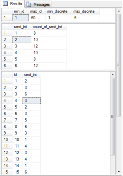
The following screen shot shows the output from the preceding script.  The output displays three result sets.

• The first result set shows the minimum and maximum values for the id and rand_int column values in the @my_randoms table variable.
• The second result set shows the observed count of die roll values.  All the observed counts are within two of the expected count value of ten over a set of sixty rolls.
• The third result set shows an excerpt of the first fifteen values in the @my_randoms table variable.

The central limit theorem, a widely known statistical principle in data science, states that the means of a sample of values from any distribution, such as a uniform distribution, is normally distributed as the number of sample means grows towards infinity (∞).  In fact, a preceding section already demonstrated that for a sample of just twenty-six sample means the central limit theorem can result in statistical conformance with a normally distributed set of observations.

Here's the script to generate twenty-six sample means from values that are known to be uniformly distributed (see the "normal distribution sample from central limit theorem.sql" file among the download files for this tip).

• The script generates twenty-six rows with ten column values on each row.  The ten column values on each row are from a uniform distribution.  These twenty-six sets of ten numbers per row are inserted into the @my_randoms table variable.
• A select statement computes the mean of the ten numbers on each row and assigns the name avg_uniform_rnd_nbr to the mean on each row.
• Because there are twenty-six sets of ten column values, there are also twenty-six means.  These twenty-six means were copied into the normal_data_with_26_obs_sample.txt file for assessment as to whether they conformed to a normal distribution.  The twenty-six means did conform to a normally distributed set of values.

-- declare local variables for passing through while loop
-- and lowest and highest values in a set of random numbers
declare 
  @loop_cntr int = 1
 ,@loop_limit int = 26
 ,@rand_int_bottom int = 18  -- lowest value in a set
 ,@rand_int_top int = 27     -- highest value in a set

-- table variable to hold int discreted random variable values
DECLARE @my_randoms table
(
   id int 
  ,rand_int_1 int
  ,rand_int_2 int
  ,rand_int_3 int
  ,rand_int_4 int
  ,rand_int_5 int
  ,rand_int_6 int
  ,rand_int_7 int
  ,rand_int_8 int
  ,rand_int_9 int
  ,rand_int_10 int
)

-- suppress rows affected message
set nocount on

-- loop for generating @loop_limit sets of 
-- of random numbers in @my_randoms
while @loop_cntr <= @loop_limit
begin

 -- populate ten columns in the @my_randoms table variable
 -- with uniformly distributed random numbers
 insert into @my_randoms
 select  
  @loop_cntr
 ,FLOOR(RAND()*(@rand_int_top-@rand_int_bottom+1))+@rand_int_bottom
 ,FLOOR(RAND()*(@rand_int_top-@rand_int_bottom+1))+@rand_int_bottom
 ,FLOOR(RAND()*(@rand_int_top-@rand_int_bottom+1))+@rand_int_bottom
 ,FLOOR(RAND()*(@rand_int_top-@rand_int_bottom+1))+@rand_int_bottom
 ,FLOOR(RAND()*(@rand_int_top-@rand_int_bottom+1))+@rand_int_bottom
 ,FLOOR(RAND()*(@rand_int_top-@rand_int_bottom+1))+@rand_int_bottom
 ,FLOOR(RAND()*(@rand_int_top-@rand_int_bottom+1))+@rand_int_bottom
 ,FLOOR(RAND()*(@rand_int_top-@rand_int_bottom+1))+@rand_int_bottom
 ,FLOOR(RAND()*(@rand_int_top-@rand_int_bottom+1))+@rand_int_bottom
 ,FLOOR(RAND()*(@rand_int_top-@rand_int_bottom+1))+@rand_int_bottom

 SET @loop_cntr = @loop_cntr + 1;

end

-- display random numbers for each row in @my_randoms table variable
-- along with mean of random numbers for each row
select 
 rand_int_1
,rand_int_2
,rand_int_3
,rand_int_4
,rand_int_5
,rand_int_6
,rand_int_7
,rand_int_8
,rand_int_9
,rand_int_10
,cast((
 rand_int_1
+rand_int_2
+rand_int_3
+rand_int_4
+rand_int_5
+rand_int_6
+rand_int_7
+rand_int_8
+rand_int_9
+rand_int_10
) as float)/10.0 avg_uniform_rnd_nbr
from @my_randoms

A set of exponentially distributed numbers can be derived from the probability density function (pdf) or the cumulative density function (cdf) of a set of exponentially distributed values; both of these functions are dependent on the same set of x values and expressions that determine the shape of any particular instance of an exponential function.  Both the pdf and cdf extend over a unit range, but the probability density function starts at 1 for the lowest possible x value of 0 and falls to a value of 0 for an x value of +∞.  In contrast, the cumulative density function starts at a value of 0 for the lowest possible x value and grows to a value of 1 for largest possible x value.  A parameter named lambda (λ) allows you to specify the shape of the pdf and cdf for any given set of x values.

Wikipedia presents these expressions for the pdf and cdf.

• The pdf has this expression.

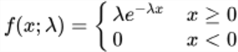
• The cdf has this expression.

You can evaluate these expressions with the exp function in SQL Server, but you may find it more convenient when you initially start working with these functions to represent their values with the exp function in Excel.  Additionally, Excel makes it easy to plot computed values.  See the "pdf and cdf for sample exponential distribution.xlsx" file for an example workbook with values for exponentially distributed values.

The next screen shot shows an Excel worksheet tab with the pdf and cdf expressions and a set of x values for interarrival times in column A.  Columns B and C contain, respectively, the pdf and cdf values based on an x value from column A and a λ of 1.  Column E contains the difference between the cdf value for the current row less the cdf value for the preceding row times 100 in an INT function.  The INT function in Excel operates like the FLOOR function in SQL Server to return the largest integer less than or equal to the specified numeric expression.  The chart to the right overlaying columns G through N displays the pdf values for each x value in rows 4 through 22.

The results in column E denote the observed count in a bin.  The bottom and top bin values for row 4 has x values of 0 and 0.0625.  The simulated count of observed events is 6 from column E on row 4.  The remaining counts for bins can be similarly derived.  The full set of non-zero observed counts were used to evaluate conformance with an exponentially distributed set of values in the last goodness-of-fit assessment example.

In my experience, the trick to getting a good set of observed counts involved manual trial and error testing for different sets of x values.  In my early tries to arrive at an exponentially distributed set of values, some intermediate bins had counts of 0.  It was relatively easy to move back and forth between deriving observed counts for bins and obtaining goodness-of-fit assessments.  I believe that I could have obtained better conformance although the reported observed counts do not differ in a statistically significant way from the expected counts for an exponential distribution with λ value of 1 and x values depicted in the following image.

Next Steps

This tip depends on several sets of files.  Twelve of these files are essential for duplicating the functionality on goodness of fit for three distribution types with two sets of data each.  An additional three files introduce you to processes for generating random numbers, such as for the three distribution types assessed for goodness of fit in this tip.  The processes for generating random numbers are useful in a general class of data science projects known as Monte Carlo simulations.

The four categories of download files for this tip include the following: core SQL files for computing the Chi Square goodness-of-fit test, a table of critical Chi Square values, sample data txt files with data that conform to and do not conform to each of the distribution types, and finally SQL and xlsx files for helping to generate sample data sets known to conform to a distribution type.  Here's a listing of the specific file names by category.

• Core SQL files for computing the Chi Square goodness-of-fit test
  • "demonstrate goodness_of_fit_for_three_different_disbributions_with_two_samples_each.sql" is the overall script file for invoking stored procedures that read data and perform the goodness-of-fit assessment with two different files for each of three distribution types.
  • "create read_from_user_file_into_##temp sp" is the script file for creating the read_from_user_file_into_##temp stored procedure.  The stored procedure can read a txt file and transfer it into a global temporary table (##temp) specified by the overall script file.
  • "create test_for_uniform_gof_in_##temp sp" is the script file for creating the test_for_uniform_gof_in_##temp stored procedure.  The stored procedure assesses how the sample values in the ##temp table conform to a uniform distribution.
  • "create test_for_normal_gof_in_##temp sp" is the script file for creating the test_for_normal_gof_in_##temp stored procedure.  The stored procedure assesses how the sample values in the ##temp table conform to a normal distribution.
  • "create test_for_exponential_gof_in_##temp sp" is the script file for creating the test_for_exponential_gof_in_##temp stored procedure.  The stored procedure assesses how the sample values in the ##temp table conform to an exponential distribution.
• The table of critical Chi Square values is included in the download for this tip as a Microsoft Excel 97-2003 Worksheet (.xls) file type with the name of "Chi Square Critical Values at 05 01 001".  Use your favorite technique for importing an Excel file into the SQL Server database from which you intend to run goodness of fit assessments.  See the "Overview of a Chi Square Goodness-of-fit test" section for additional specifications for importing the xls file.
• There are six files in the download for this tip that include sample data sets for performing assessments with the overall script.
  • The raw_data_for_uniform_test_based_on_en_wikipedia.txt file contains data from Wikipedia that fail to pass the assessment for a uniformly distributed set of values.
  • The uniform_fair_die_rolls_sample.txt file contains freshly generated data from the SQL Server rand function to simulate 60 die rolls; the data in this file passes the assessment for a uniformly distributed set of values.
  • The raw_data_for_normality_test_excelmasterseriesblog.txt file contains data from the Excel Master Series blog that fail to pass the assessment for a normally distributed set of values.
  • The normal_data_with_26_obs_sample.txt file contains freshly generated data with sample means based on the SQL Server rand function to simulate a normal distribution; the data in this file passes the assessment for a normally distributed set of values.
  • The processor_lifetime_days_wo_header.txt file contains data from professor Kendall Nygard's lecture note on assessing the goodness of fit of lifetime duration times for processors to an exponential distribution.  The data in the file fail to pass the assessment for an exponentially distributed set of values.
  • The raw_data_exponential_with_lambda_of_1.txt file contains freshly generated data from a manual iterative process to generate exponentially distributed value; the data in this file passes the assessment for an exponentially distributed set of values.
• Three remaining files help to illustrate processes for generating values conforming to a distribution type.  These files are described fully in the "Code and process review for random number generation based on distribution types" section of this tip.  Their names are: "uniform distribution fair die sample.sql", "normal distribution sample from central limit theorem.sql", and "pdf and cdf for sample exponential distribution.xlsx".

The download file for this tip includes the fifteen files referenced in this section. After getting the overall script file demonstration to work as described in the tip, you should be equipped to participate in a data science project where you are charged with assessing goodness of fit for uniformly, normally, or exponentially distributed values.  Additionally, you will have a framework that is suitable for expansion to other kinds of distributions.

About the author

Rick Dobson is an author and an individual trader. He is also a SQL Server professional with decades of T-SQL experience that includes authoring books, running a national seminar practice, working for businesses on finance and healthcare development projects, and serving as a regular contributor to MSSQLTips.com. He has been growing his Python skills for more than the past half decade -- especially for data visualization and ETL tasks with JSON and CSV files. His most recent professional passions include financial time series data and analyses, AI models, and statistics. He believes the proper application of these skills can help traders and investors to make more profitable decisions.

This author pledges the content of this article is based on professional experience and not AI generated.

View all my tips