By: Rick Dobson | Updated: 2022-01-21 | Comments | Related: > TSQL
Problem
Show how to model time series trends and reversals with T-SQL and logs. Present a framework with the models about when to initiate actions based on reversals in time series.
Solution
Time series often demonstrate periods of sustained increases (uptrend) or decreases (downtrend). The transition from an uptrend to a downtrend (or vice versa) is known as a reversal. In general, things do not go up (or down) forever. Times series reversals often signal when an action becomes appropriate. At the start of a rainy season, it is a good idea for a retail store to keep umbrellas and rain jackets in stock. Another example is for electric utilities to turn on or off swing capacity generators depending on the demand during a time of day or a season of the year. This course of action can help to provide inexpensive rates to utility rate payers.
One way to spot a reversal is by examining moving averages. When a moving average with a shorter period length starts to exceed a moving average with a longer period length, the time series indicate a reversal. The reversal is from a downtrend to an uptrend. In contrast, when a moving average with a longer period length starts to exceed a moving average with a shorter period length, a downtrend has begun.
This tip demonstrates some models for detecting the start of periods of rising or falling financial securities prices based on exponential moving averages. The demonstration is simplified because it relies on a log to keep track of time series values as well as exponential moving averages with different period lengths. As a SQL Server professional, you are likely to be familiar with use of logs for tracking SQL Server performance. You can use logs in a similar way for comparing different time series models about when it is best to perform some action, such as buy or sell a stock.
About the data for this tip
The data for this tip draws on two tables (stooq_prices and denormalized_emas). The data in both tables contains results for six financial securities with symbols of AAPL, GOOGL, MSFT, SPXL, TQQQ, and UDOW.
The stooq_prices table is a typical table of price and volume data for financial securities over time. The table contains a separate row for each symbol on each trading day. The data for each row contains open, high, low, and close prices as well as the number of shares traded for a security on a date. The process for collecting this kind of price and volume data from the Stooq web site is described in a prior tip.
Here is a short script that shows how to display the first and last five rows for the symbol of one financial security in the data source for this tip; the security is Apple, whose symbol is AAPL. This tip assumes the data resides in the DataScience database. You can use any other database you prefer so long as you populate the database properly with time series data.
use [DataScience]
go

-- display first and last five rows for a symbol in stooq_prices
declare @symbol nvarchar(10) = 'AAPL'

select top 5
       [date]
      ,[symbol]
      ,[open]
      ,[high]
      ,[low]
      ,[close]
      ,[volume]
from [DataScience].[dbo].[stooq_prices]
where symbol = @symbol

select
       [date]
      ,[symbol]
      ,[open]
      ,[high]
      ,[low]
      ,[close]
      ,[volume]
from [DataScience].[dbo].[stooq_prices]
where symbol = @symbol
and date between '2021-06-24' and '2021-06-30'
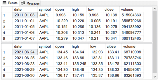
Here are some excerpts from the results set from the preceding script segment.
- The top pane is for the first five rows whose first trading date is January 3, 2011, the first trading date in 2011.
- The bottom pane is for the last five rows whose final trading date is June 30. 2021, the last trading date in the first half of 2021.
- This tip will use two numeric columns from the stooq_prices table.
- The close column shows the final price during a trading date for a security.
- The open column shows the initial price during a trading date for a security.
Here is a second script segment to show the first and last five rows from the denormalized_emas table for the AAPL symbol. The full script runs from the DataScience database.
-- display first and last five rows for a symbol in denormalized_emas
declare @symbol nvarchar(10) = 'AAPL'

select top 5
    date
       ,symbol
   ,denormalized_emas.ema_10
       ,denormalized_emas.ema_20
       ,denormalized_emas.ema_30
       ,denormalized_emas.ema_50

from denormalized_emas
where symbol = @symbol

select top 5
    date
   ,symbol
   ,denormalized_emas.ema_10
       ,denormalized_emas.ema_20
       ,denormalized_emas.ema_30
       ,denormalized_emas.ema_50

from denormalized_emas
where symbol = @symbol
and date between '2021-06-24' and '2021-06-30'
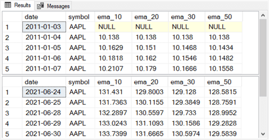
Here is an image showing some excerpts from the results set from the preceding script.
- Notice the first date from the top pane and the last date from the bottom pane match those from the stooq_prices table.
- The values in each ema column are for different period lengths of 10, 20, 30, and 50.
- Because exponential moving averages are undefined for the first value in an underlying time series, the ema values in the first row are all NULL.
- Also, the second row of ema values are all equal to 10.138. This again is by definition from the algorithm used to compute exponential moving averages.
- The T-SQL code to compute and display exponential moving averages in a denormalized format appears in this prior tip. The prior tip fully explains the process of storing ema values in normalized and denormalized format; the download for this tip also includes code for computing ema values for underlying time series values and storing them in a denormalized format.
A T-SQL framework for computing buy and sell dates and logging the dates and prices
All the models examined in this tip involve a cross-over of exponential moving averages with different period lengths. This tip’s initial model issues signals about when to buy and sell a financial security based on ten-period length and thirty-period length exponential moving averages. This initial example is meant to serve as a framework for evaluating how other sets of ema values perform for signaling buy and sell dates. Also, with slight modifications to the T-SQL framework in this section, you can evaluate how different assumptions about sets of ema values perform for signaling buy and sell dates.
When a ten-period length exponential moving average (ema) rises and crosses above a thirty-period length ema, the underlying prices are beginning to increase. Rising prices for close prices can eventually cause ema sets with a shorter period length to increase from below to above ema sets with a longer period length. The larger the price increase and the longer the duration of rising prices, the greater the shorter period length ema set will gain on the longer period length ema set.
Here are the specifications for the first model in this tip.
- Issue a buy signal when a ten-period length ema rises above a thirty-period length ema following one or more consecutive periods in which a thirty-period length ema is greater than a ten-period length ema.
- Issue a sell signal when a ten-period length exponential moving average falls below or equal to a thirty-period length ema.
- At the end of each trading day, the T-SQL code for implementing the model writes out the prices, exponential moving averages, as well as either a buy or sell signal (if appropriate).
- When a signal is issued, it is to buy or sell a security on the next trading date. This is because a cross-over cannot be known until after the close of trading for a day.
The T-SQL code for implementing the first model in this tip appears below. The code resides in the raw_log_for_rising_and_falling_below_30.sql file, which is in this tip’s download. There are two main parts to the script inside the file.
- A subquery named for_buy_sell_log_for_ema_10_vs_30 pulls and joins data from the stooq_prices and denormalized_emas tables based on matching symbol and date values. The results set from the inner query becomes the data source for the outer query.
- The outer query implements the model specification based on the data from
the inner query.
- A select statement returns selected values from the inner query.
- The select query includes two case statements for computing critical
values that can be saved in a log for the model.
- The first case statement computes buy and sell signals based on the model’s specification
- The second case statement retrieves the buy or sell price, respectively, for a buy or sell signal
- The results set from the outer select statement can optionally be held in a table that stores the model’s log of buy and sell actions. This part of the script is commented out to keep the focus on the model’s logic. For the purposes of this demonstration, the log is manually saved.
use [DataScience]
go

select
 date
,symbol
,[open]
,[close]
,ema_10_lag_1
,ema_30_lag_1
,ema_10
,ema_30

-- set buy and sell signals
,case
   when ((ema_10_lag_1 <= ema_30_lag_1) and  (ema_10 > ema_30)) then 'buy signal'
   when ((ema_10_lag_1 >= ema_30_lag_1) and (ema_30 > ema_10)) then 'sell signal'
   else null
 end buy_sell_signal

-- set buy and sell prices
,case
   when ((ema_10_lag_1 <= ema_30_lag_1) and  (ema_10 > ema_30)) then open_lead_1
   when ((ema_10_lag_1 >= ema_30_lag_1) and (ema_30 > ema_10)) then open_lead_1
   else null
 end buy_sell_price

--into dbo.falling_below_30_log

from
(
-- source rows for buy/sell actions
select
 stooq_prices.*
,denormalized_emas.ema_3
,denormalized_emas.ema_10
,denormalized_emas.ema_30
,denormalized_emas.ema_50
,denormalized_emas.ema_200
,lag(denormalized_emas.ema_10,1) over (partition by stooq_prices.symbol
     order by denormalized_emas.date) ema_10_lag_1
,lag(denormalized_emas.ema_30,1) over (partition by stooq_prices.symbol
     order by denormalized_emas.date) ema_30_lag_1
,lead(stooq_prices.[open],1) over(partition by stooq_prices.symbol
      order by  denormalized_emas.date) open_lead_1
from stooq_prices
inner join denormalized_emas
on stooq_prices.date = denormalized_emas.date and stooq_prices.symbol = denormalized_emas.symbol
) for_buy_sell_log_for_ema_10_vs_30
To understand the performance of the model predictions about when to buy and sell stocks, you must learn to read the log of model activity.
- The buy and sell signal dates indicate when and at what price the model designates the buying and selling of a security.
- The first sell signal to follow a buy signal completes a buy-sell cycle.
- Only sell signals with a preceding buy signal belong to a buy-sell cycle.
- Similarly, a buy signal without a following sell signal does not belong to a buy-sell cycle.
- A sell signal without a preceding buy signal and a buy signal without a trailing sell signal are most likely to occur at beginning and end of a time series, but they can happen at other points in a time series depending on the model rules for buy and sell signals as well as the time series data.
- You can assess changes in the price of a security during a buy-sell cycle
by comparing buy and sell prices.
- The change in the price of a security during a buy-sell cycle is its
sell price less its preceding buy price.
- A winning trade for a buy-sell cycle has a positive change in price.
- A losing trade for a buy-sell cycle has a negative change in price.
- The rate of change in the price of a security during a buy-sell cycle is the change in the price of a security divided by the buy price of the security’s buy-sell cycle.
- The annual rate of change represents the rate of change for a buy-sell
cycle if the percent change during a cycle adjusted for its duration in
trading days occurred over a whole year. You can compute the annual
rate of change as
- The rate of change divided by the number of trading days during a buy-sell cycle
- Multiplied by the number of trading dates in a year (about 250)
- The annual rate of change makes it possible to compare the price impact during buy-sell cycles with different durations
- The change in the price of a security during a buy-sell cycle is its
sell price less its preceding buy price.
Here are some sequential excerpts from the log of the initial model for Apple (AAPL) during a period of particular interest. The period starts in mid-June 2019 and runs through mid-September 2020. Our initial model issues three buy signals for AAPL during this span of time. The most interesting stock market event during this span of time was the coronavirus crash of late February 2020 through very early in April 2020. According to Wikipedia, the start of the stock market crash was 2020-02-20, and the last day of the crash was 2020-04-07. One mark of success for the model was that it did not issue buy signals for Apple during the coronavirus crash. The model’s sole sell signal during the crash was issued in the first week of the crash.
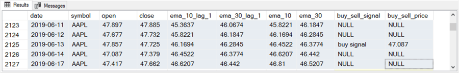
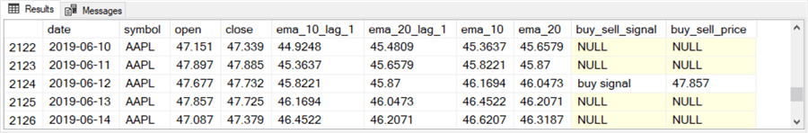
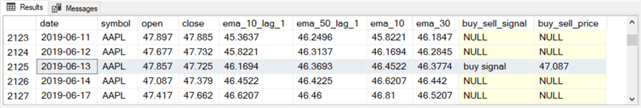
The following screen shot shows the buy signal for the first buy-sell cycle. The model issued a buy signal for the AAPL symbol after the market closed on 2019-06-13.
- You can note that the ema_10 moves from below ema_30 on 2019-06-12 to above ema_30 on 2019-06-13. This fact cannot be confirmed until after the market closes on 2019-06-13 because the ema_10 and the ema_30 for 2019-06-13 requires a close price.
- Consequently, the buy signal issued on 2019-06-13 cannot be responded to until the opening of the market on 2019-06-14. The buy_sell price (47.087) for the buy_sell signal corresponds to the open price on 2019-06-14.
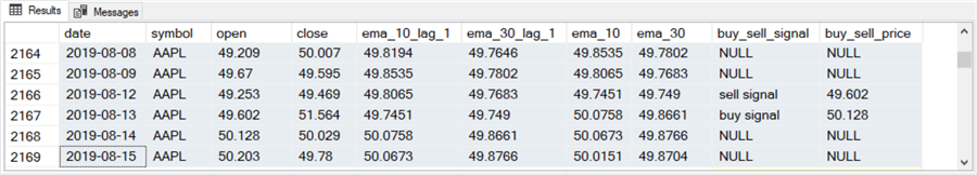
The next log excerpt shows the sell-signal row for 2019-08-12. On the next trading date (2019-08-13), the model issues a new buy signal to start a new buy-sell cycle.
- The 2019-08-12 sell signal has a sell price of 49.602 for the open on 2019-08-13. The buy-sell cycle from the 2019-06-14 open price through the open price on 2019-08-13 results in a gain of 2.515 per AAPL share (49.602 – 47.087). This gain corresponds to a percentage change of about 5.3 % over 2 months or an annual change rate of about 31.8%.
- The buy signal on the 2019-08-13 indicates the start of a new buy-sell cycle starting with the market open on 2019-08-14.
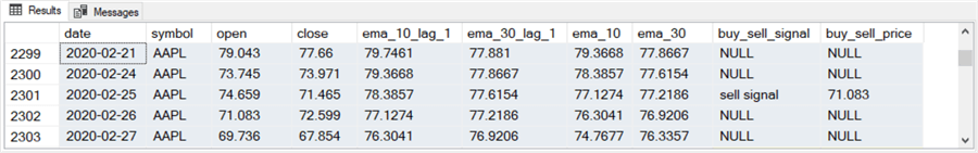
The sell signal for the buy signal in the preceding log excerpt occurs on 2020-02-25. This date is especially significant because it occurs just after the onset of the coronavirus stock market crash with a sell price of 71.083 during the market open on 2020-02-26. The change in price per share for the buy-sell cycle is 20.955 (71.083 – 50.128). You can compute the rate of change as 41.8% over the buy-sell cycle, and the annual rate of change as about 83.6%.
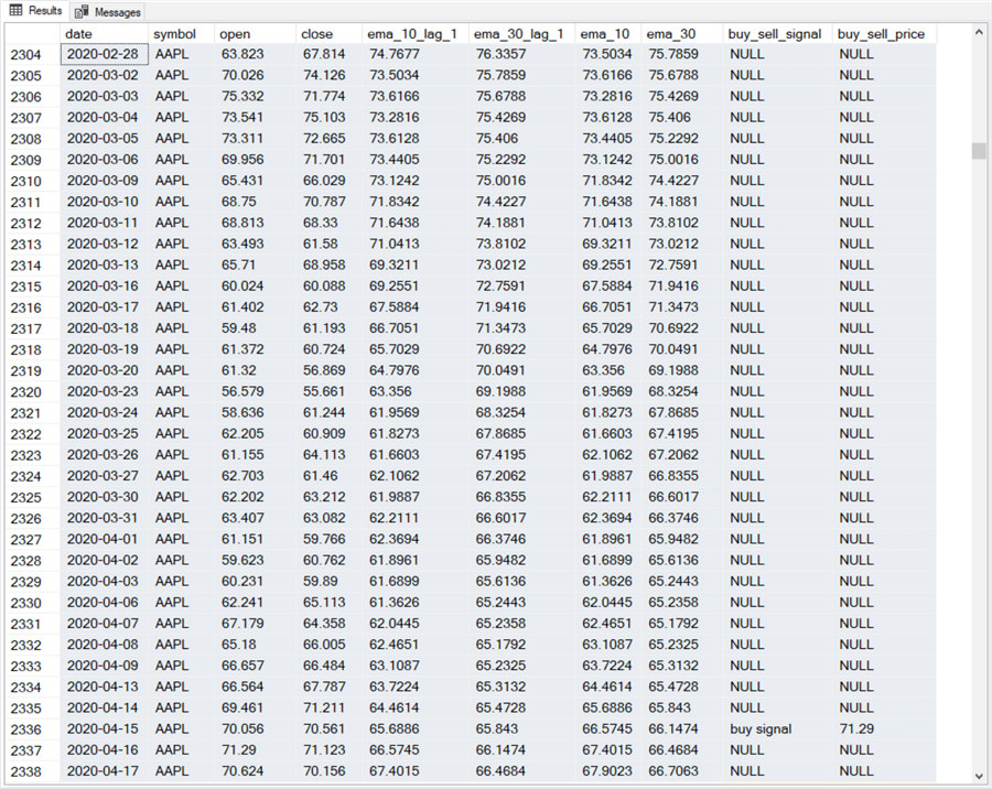
The third buy signal for the AAPL symbol in the sequence of trades logged here does not show until the row for 2020-04-15. One especially important point to note about the buy signal is that the model does not issue it until after the end of the coronavirus stock market crash. In other words, the model avoids issuing a buy signal during the crash. In fact, the model does not issue a buy signal until about one week after the crash ends (2020-04-07).
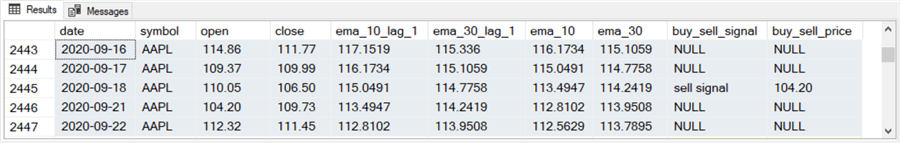
The final log excerpt for this sequence of trades shows the sell signal for the preceding buy signal was issued on 2020-09-18, which is executed on the next trade date of 2020-09-21. The price change during the buy-sell cycle was 32.91 (104.20 – 71.29). The percent change during the cycle was 46.2%, which equates to an annual rate of change of about 110.9%.
Models and logs for ema_10 versus ema_20 and ema_10 versus ema_50
This section presents code excerpts and log excerpts for two additional models that are based on simple variations of the model in the preceding section. The model in the preceding section decides whether to issue buy and sell signals by comparing ema_10 to ema_30 both in the preceding period and the current period.
- The rules for assigning a buy signal are that ema_10 must be less than or equal to ema_30 in the preceding period and then ema_10 must move to being greater than ema_30 in the current period.
- The rules for assigning a sell signal are that ema_10 must be greater than or equal to ema_30 in the preceding period and then ema_10 must move to being less than ema_30 in the current period.
The two models in this section decide whether to issue buy and sell signals by replacing ema_30 in the preceding model with either ema_20 or ema_50.
The alternative two models in this section combined with the model in the preceding section facilitates a sensitivity analysis for how far you must be away from ema_10 when searching for an effective ema set for finding reversals. Also, different comparison exponential moving averages versus ema_10 filter the data so that special cleaning and processing rules are required for the logs.
Here is the most important special code for the model comparing ema_10 to ema_20. This code excerpt for the ema_10 versus the ema_20 model sets the buy and sell signals as well as the associated buy and sell prices. The only difference between the code below for this model and the code in the previous section is the replacement of ema_30 with ema_20. This replacement process also pertains to lagged values, such as ema_20_lag_1. You additionally must make sure that ema_20 and ema_20_lag1 are available from the source data subquery at the bottom of the script (open_lead_1).
-- set buy and sell signals
,case
   when ((ema_10_lag_1 <= ema_20_lag_1) and  (ema_10 > ema_20)) then 'buy signal'
   when ((ema_10_lag_1 >= ema_20_lag_1) and (ema_20 > ema_10)) then 'sell signal'
   else null
 end buy_sell_signal

-- set buy and sell prices
,case
   when ((ema_10_lag_1 <= ema_20_lag_1) and  (ema_10 > ema_20)) then open_lead_1
   when ((ema_10_lag_1 >= ema_20_lag_1) and (ema_20 > ema_10)) then open_lead_1
   else null
 end buy_sell_price
The changes for a model comparing ema_10 to ema_50 are like those for comparing ema_10 to ema_20. For example, the code for issuing buy and sell signals as well as specifying the buy price and sell price have the format in the following code excerpt. You additionally need to update the source data query by replacing ema_30 and ema_30_lag_1 with ema_50 and ema_50_lag_1.
-- set buy and sell signals
,case
   when ((ema_10_lag_1 <= ema_50_lag_1) and  (ema_10 > ema_50)) then 'buy signal'
   when ((ema_10_lag_1 >= ema_50_lag_1) and (ema_50 > ema_10)) then 'sell signal'
   else null
 end buy_sell_signal

-- set buy and sell prices
,case
   when ((ema_10_lag_1 <= ema_50_lag_1) and  (ema_10 > ema_50)) then open_lead_1
   when ((ema_10_lag_1 >= ema_50_lag_1) and (ema_50 > ema_10)) then open_lead_1
   else null
 end buy_sell_price
The complete T-SQL code for both models referenced in this section as well as all other sections is available in the download file for this tip.
When you are comparing different exponential moving averages with different period lengths, your buy and sell signal dates and their corresponding buy and sell prices can change between models. In addition, any given buy-sell cycle may include more than one buy signal and one sell signal. This is not an error. To keep the code for a model easy to read, this tip does not include code for ensuring
- there is just one buy signal per buy-sell cycle and
- there is just one sell signal per buy-sell cycle
Always ignore any repeat buy signals after the first buy signal in a buy-sell cycle before you encounter the first sell signal. Likewise, ignore any repeat sell signals after the first sell signal trailing a first buy signal in a buy-sell cycle. The last model in this tip illustrates one example of how to obtain repeat sell signals.
Because this tip is just introducing modeling and logging time series models with T-SQL, repeat buy signals and repeat sell signals are manually handled. A soon to be published article "Use Cases for While and Goto Loops with T-SQL for Time Series Data" presents T-SQL code for filtering the log for a model by programmatically implementing these log-handling guidelines. The script implementing the guidelines can extract from the raw log just the buy signals and the sell signals for a succession of buy-sell cycles.
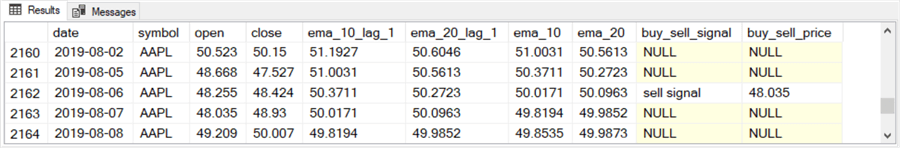
The following pair of screen shots show the buy signal and sell signal for a buy-sell cycle pointing to a buy on 2019-06-13 and a sell on 2019-08-07. You can see from the column headers that these log excerpts are for the model comparing ema_10 to ema_20. If you examine the log excerpts from the prior section for the model comparing ema_10 to ema_30 to this model, which relies on ema_10 and ema_20, you can see the buy and sell dates and prices are very similar.
- This section’s model has a buy signal on 2011-06-12 pointing to a buy action on 2011-06-13. The prior section’s model issues a buy signal on 2011-06-13 pointing to a buy action on 2011-06-14. This section’s model issues a buy signal one day before the model from prior section.
- Similarly, this section’s model issues a sell signal on 2019-08-06, which is several days before the closest sell signal from the prior section’s model. The closest sell signal date for the prior section is on 2019-08-12.
- The price change for these highly similar buy and sell dates is
- 0.508 (48.035 – 47.527) per share for the model from this section and
- 2.515 (49.602 – 47.087) per share for the model from the prior section
- The model from the prior section, which picks buy and sell dates based on ema_10 and ema_30, selected buy and sell points with a price change that is about five times greater than the ema_10 and ema_20 model from this section. A statistical comparison of the logs from both models can confirm if the ema_10 and ema_30 model is generally superior to the ema_10 and ema_20 model across the full set of buy-sell cycles from the logs.
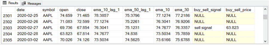
The next pair of screen shots show first and last dates from log excerpts from the model comparing ema_10 and ema_50. This model is evaluated from the same starting date (mid-June 2019) as the two preceding model comparisons for ema_10 and ema_30 as well as for ema_10 versus ema_20.
- In this case, the buy signal row is 2019-06-13. The buy price is 47.087, which is the open price on 2019-06-14. This outcome exactly matches the buy signal date and price as set by the ema_10 and ema_30 model in the preceding section.
- The only sell signal row after the initial row for the buy-sell cycle occurs on 2020-02-27. This is nearly eight months after the start date for the buy-sell cycle! The sell price for the last date in the cycle is 63.823.
- The performance statistics per for this buy-sell cycle are as follow
- The price change is 16.736 (63.823 – 47.087)
- The percent price change is 35.5% (16.736/47.087)
- The annual percent change is about 53.3%
Two main purposes of this tip are to introduce you to the logs from each model and show the application of some methods for comparing results across models. Subsequent tips will present more detailed analytical comparisons across multiple models for multiple symbols in a search for guidelines about when to use each model.
A model with asymmetric buy and sell cross-over points
The models considered so far in the tip specified symmetric cross-over points for buy and sell signals. That is, the exact same pair of exponential moving averages were examined for a cross-over to determine whether to issue both buy and sell signals. In this section, different pairs of exponential moving averages are used for issuing buy versus sell signals.
When comparing a pair of exponential moving averages for a cross-over, the shorter the period length of the two exponential moving averages, the faster the buy or sell signal is issued. In this section, a pair of exponential moving averages with shorter period lengths are checked for a cross-over before issuing a sell signal than before issuing a buy signal. Therefore, the sell signal is issued faster than the buy signal. By issuing a sell signal sooner, the model in this section may be able to exit trades sooner than those in the preceding section. If the descent from a peak value in a buy-sell cycle is very steep, such as for securities with high volatility, then a model like the one in this section may be preferable to those in the preceding section.
An example of the specification for a model with asymmetric buy and sell cross-over points appears below.
- A buy signal is issued when ema_10 is greater than ema_30 (so long as ema_10_lag_1 is less than or equal to ema_30_lag_1).
- On the other hand, a sell signal is issued when ema_3 is less than ema_10 (so long as ema_10_lag_1 is greater than or equal to ema_30_lag_1).
- Because the issuance of a sell signal depends on a cross-over of ema_3 and ema_10, the sell signal is issued faster than the buy signal which depends on a cross-over of ema_10 and ema_30.
use [DataScience]
go

select
 date
,symbol
,[open]
,[close]
,ema_3_lag_1
,ema_10_lag_1
,ema_30_lag_1
,ema_3
,ema_10
,ema_30

-- set buy and sell signals
,case
   when (
         (ema_10_lag_1 <= ema_30_lag_1) and  (ema_10 > ema_30)
       )
          then 'buy signal'
   when (
         ((ema_10_lag_1 >= ema_30_lag_1) and (ema_3 < ema_10))
       )  then 'sell signal'
   else null
 end buy_sell_signal

-- set buy and sell prices
,case
   when (
         (ema_10_lag_1 <= ema_30_lag_1) and  (ema_10 > ema_30)
       )  then open_lead_1
   when (
         ((ema_10_lag_1 >= ema_30_lag_1) and (ema_3 < ema_10))
       )  then open_lead_1
   else null
 end buy_sell_price

--into dbo.falling_below_10_or_30_log

from
(
-- source rows for buy/sell actions
select
 stooq_prices.*
,denormalized_emas.ema_3
,denormalized_emas.ema_10
,denormalized_emas.ema_30
,denormalized_emas.ema_50
,denormalized_emas.ema_200
,lag(denormalized_emas.ema_3,1) over (partition by stooq_prices.symbol
      order by denormalized_emas.date) ema_3_lag_1
,lag(denormalized_emas.ema_10,1) over (partition by stooq_prices.symbol
      order by denormalized_emas.date) ema_10_lag_1
,lag(denormalized_emas.ema_30,1) over (partition by stooq_prices.symbol
      order by denormalized_emas.date) ema_30_lag_1
,lead(stooq_prices.[open],1) over(partition by stooq_prices.symbol
      order by  denormalized_emas.date) open_lead_1

from stooq_prices
inner join denormalized_emas
on stooq_prices.date = denormalized_emas.date
and stooq_prices.symbol = denormalized_emas.symbol
) for_buy_sell_log_for_ema_10_vs_30
The next screen shot shows a results set excerpt for the rows starting around 2019-06-13 from the preceding script. This log excerpt exactly matches the first script which had symmetric cross-over criteria for buy signals and sell signals. Both excerpts show a buy signal row on 2019-06-13 with a buy_sell_price value of 47.087 for the open of trading on 2019-06-14
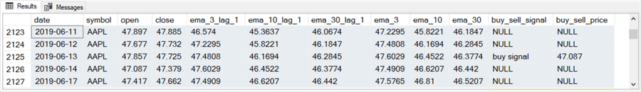
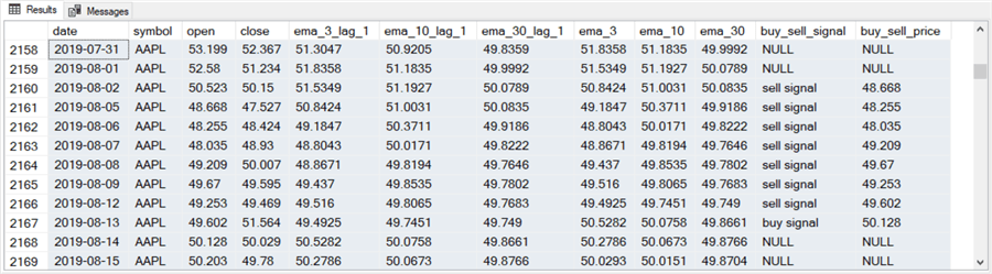
The final screen shot of this tip, which appears next, presents rows from around the sell signal matching the buy signal in the preceding script.
- Note that there are eight rows that include sell signal in the buy_sell_signal column. This may be because the period preceding the current period and the current period have different criteria for the sell signal.
- Because the first sell signal row is on 2019-08-02, the open price on the next row (with a date of 2019-08-05) completes the buy-sell cycle.
- The seven other rows in the screen shot below with a sell signal value in the buy_sell_signal column are merely rows that match the criteria for a sell signal, but none of these other rows are the first row with a sell signal value after the buy signal row in the preceding screen shot.
- Perhaps the most important point about the screen shot below is that sell signal date and price is different in the model from this section than the model from the initial model in this tip. This is because of the use of an asymmetric cross-over setting in the script for this section as opposed to the use of a symmetric cross-over setting in the script for the initial model.
- In addition, the sell signal date occurs more closely to the buy signal than in the initial model in this tip. This is because the sell signal cross-over is for ema_3 versus ema_10 in the model for this section compared to a cross-over comparison of ema_10 versus ema_30 for the initial model.
Next Steps
This tip’s download file contains eleven files to help you get a hands-on feel for using T-SQL for downloading to SQL Server historical price and volume data from the Stooq website.
- Six of the files are the csv files.
- The two most critical files for re-running the code as described in this tip are named stooq.csv, which is for populating the stooq_prices table in SQL Server, and denormalized_emas.csv, which is for populating the denormalized_emas table in SQL Server. These files contain historical price and volume data as well as ema data in denormalized format for six symbols (AAPL, GOOGL, MSFT, SPXL, TQQQ, UDOW).
- The other four csv files contain the logs – one for each of the four models.
- Five .sql file are also in the download for this tip.
- There is one .sql file for each of the four models in this tip.
- There is also one file with T-SQL code that you may find helpful for computing the denormalized emas from the stooq_prices table. Recall that the "About the data for this tip" section also includes a link to a prior tip with an additional example on how to compute emas in normalized and denormalized formats.
After verifying the code works as described with the sample data files, you are encouraged to use other date ranges and/or symbols than those reported on in this tip. Practice reading the logs for whatever changes you make to the code. Confirm your ability to verify that any changes you make to the code match those in the generated log file from the new model.


About the author
 Rick Dobson is an author and an individual trader. He is also a SQL Server professional with decades of T-SQL experience that includes authoring books, running a national seminar practice, working for businesses on finance and healthcare development projects, and serving as a regular contributor to MSSQLTips.com. He has been growing his Python skills for more than the past half decade -- especially for data visualization and ETL tasks with JSON and CSV files. His most recent professional passions include financial time series data and analyses, AI models, and statistics. He believes the proper application of these skills can help traders and investors to make more profitable decisions.
This author pledges the content of this article is based on professional experience and not AI generated.
View all my tips
Article Last Updated: 2022-01-21