Advanced Databricks Lakehouse Encryption, Security, Query Plans, CDC

By: Ron L'Esteve | Updated: 2022-05-10 | Comments | Related: > Azure Databricks

Problem

There are many advantages to implementing a Data Lakehouse including separation of low-cost modularized storage from pay-as-you-go and reserved instance compute; easy access to high-powered AI and Machine Learning resources; and secure data sharing and streaming analytics capabilities. Many organizations are adopting the Data Lakehouse Paradigm with several technologies including Databricks. As customers continue their deeper research and analysis of Lakehouse capabilities, they are seeking to understand the advanced capabilities of Databricks, specifically, around dynamically handling Data Encryption, data and query profile capabilities, how constraints are handled in Databricks notebooks, and how to get started with Change Data Capture (CDC) using Delta Live Tables (DLT) Merge.

Solution

In this article, you will learn more about some of the advanced capabilities of Databricks such as Dynamic Data Encryption for encrypting and decrypting data with the built-in aes_encrypt() and aes_decrypt() functions, including how you can integrate this with row-level security by using the is_member() function. You will also learn about how to profile your data distributions and compute summary statistics which can be visualized on an exploratory basis within your notebook. Query Profile within the SQL Analytics Workspace to visually view your query plans will also be explained. Finally, you will learn more about Delta Live Tables (DLT), which are an abstraction on top of Spark that enables you to write simplified code to apply SQL MERGEs and Change Data Capture (CDC) to enable upsert capabilities on DLT pipelines with Delta format data.

Dynamic Data Encryption

Encrypting and Decrypting data is a critical need for many organizations as part of their data protection regulations. With the new Databricks runtime 10.3, there are two new functions, aes_encrypt() and aes_decrypt(), that serve this very purpose. They can be combined with row-level security features to only display the decrypted data to those who have access.

The function works by simply writing a SQL statement like the following code by specifying what to encrypt as well as a 32bit encryption key: SELECT aes_encrypt('MY SECRET', 'mykey'). To decrypt your data, simply run the aes_decrypt () function with code that is similar to the following, which wraps your encrypted value and key within the decrypt function and casts it as a string: SELECT CAST(aes_decrypt(unbase64('encryptedvalue'), 'mykey') as string).

For scenarios where you are seeking to add row-level security-based decryption, you could start by creating the following tables shown in the figure below. The first table, tbl_encrypt, contains the encryption key used in the encryption function and group name which matches the name of the corresponding security groups that have been in the Databricks Admin UI. The next table, tbl_data, contains the data that needs to be protected along with the same group name that can be mapped to tbl_encrypt.

The is_Member function can be used as a filter in a SQL statement to only retrieve rows which the current user has access. The following SQL code creates a view on tbl_encrypt to only show groups that a user has access to.

CREATE VIEW vw_decrypt_data
AS
SELECT * FROM tbl_encrypt 
WHERE is_Member(group_name)

Finally, you could write another SQL query like the following to decrypt your data dynamically based on the group that you have row-level access. Additionally, if an encryption key is ever deleted from tbl_encrypt, then the following query will return 'nulls' for the rows that you may still have access to but since the encryption is no longer part of the lookup table, you will not be able to decrypt the data and will only see 'nulls' in place of the actual data. This pattern prevents the need from having to store duplicate versions of data by dynamically decrypting row-level data based on group-based membership.

SELECT
   cast(aes_decrypt(a.name, DA.encryption_key) as string) Name,
   cast(aes_decrypt(a.email, DA.encryption_key) as string) Email,
   cast(aes_decrypt(a.ssn, DA.encryption_key) as string) SSN,
FROM
   tbl_data a
   LEFT JOIN vw_decrypt_data b ON a.group_name = b.group_name

Data Profile

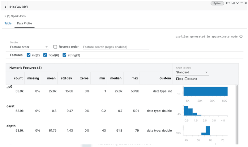
Within Databricks notebooks, data distributions and computing summary statistics can be visualized on an exploratory basis directly by running the display(df) command to display the data frame within a notebook as part of the data profiling feature within the notebooks. This can be seen in the figure shown below, where a data profile will be generated in the data frame across the entire dataset to include summary statistics for columns along with histograms of the columns' value distributions.

Query Profile

The Databricks Data Engineering and Data Science workspaces provide a Databricks UI including visual views of query plans and more. The SQL Analytics Workspace provides the ability to view details on Query History. In addition, it provides a nice feature to profile your SQL Queries in detail to identify query performance bottlenecks and performance optimization opportunities. These details include multiple graphs, memory consumption, rows processed, and more which can also be downloaded and shared with others for further analysis.

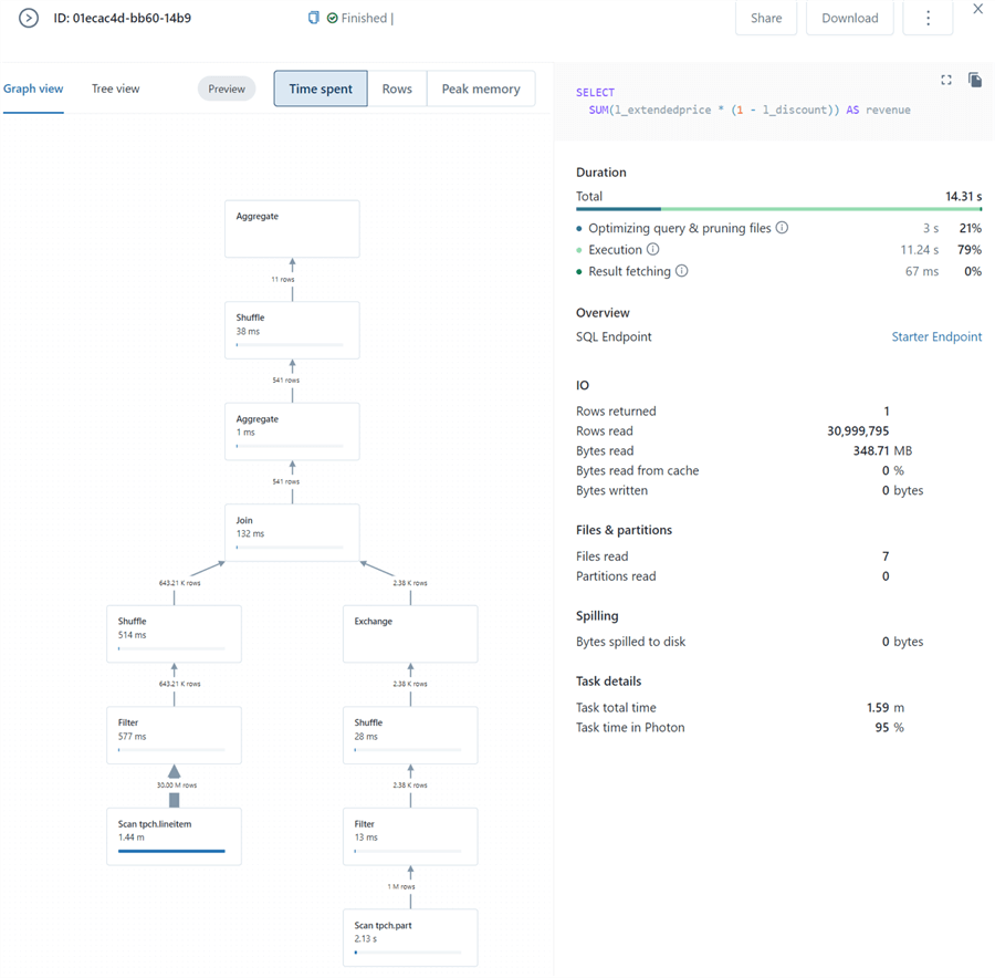
For example, within the Databricks Data Engineering Workspace, I run a sample SQL Query using a small Starter Endpoint on the sample tpch data that is included with the workspace, as shown in the figure below.

New Tpch query in SQL Analytics Workspace

Here is the sample SQL Query which I ran in the Databricks SQL Analytics Workspace:

SELECT
     SUM(l_extendedprice* (1 - l_discount)) AS revenue
FROM
     samples.tpch.lineitem,
     samples.tpch.part
WHERE
     (
      p_partkey = l_partkey
      AND p_brand = 'Brand#12'
      AND p_container IN ('SM CASE', 'SM BOX', 'SM PACK', 'SM PKG')
      AND l_quantity >= 1 AND l_quantity <= 1 + 10
      AND p_size BETWEEN 1 AND 5
      AND l_shipmode IN ('AIR', 'AIR REG')
      AND l_shipinstruct = 'DELIVER IN PERSON'
     )
     OR
     (
      p_partkey = l_partkey
      AND p_brand = 'Brand#23'
      AND p_container IN ('MED BAG', 'MED BOX', 'MED PKG', 'MED PACK')
      AND l_quantity >= 10 AND l_quantity <= 10 + 10
      AND p_size BETWEEN 1 AND 10
      AND l_shipmode IN ('AIR', 'AIR REG')
      AND l_shipinstruct = 'DELIVER IN PERSON'
     )
     OR
     (
      p_partkey = l_partkey
      AND p_brand = 'Brand#34'
      AND p_container IN ('LG CASE', 'LG BOX', 'LG PACK', 'LG PKG')
      AND l_quantity >= 20 AND l_quantity <= 20 + 10
      AND p_size BETWEEN 1 AND 15
      AND l_shipmode IN ('AIR', 'AIR REG')
      AND l_shipinstruct = 'DELIVER IN PERSON'
     )

As a next step, when you navigate to the 'Query History' tab and click on 'View Query Profile', you will be able to see the detailed query profile, as shown in the figure below. You will have the option to toggle between either graph or tree view. Also, you can view these details by time spent, rows, or peak memory. Towards the right, you can see the duration, IO, files, partitions, spilling, and task details. Finally, you can easily share or download this query plan with a click of a button.

Constraints

Delta Tables in Databricks support SQL constraint management clauses including NOT NULL and CHECK to ensure data quality and integrity is automatically verified. Upon violation of constraints, the InvariantViolationException will be thrown when new data cannot be added.

For the NOT NULL constraint, you can add this within the create table statement's schema definition, as shown in the code below.

CREATE TABLE Customers (
    id INT NOT NULL,
    FirstName STRING,
    MiddleInitial STRING NOT NULL,
    LastName STRING,
    RegisterDate DATETIME
  ) USING DELTA;

You can also drop a NOT NULL constraint or add a new NOT NULL constraint by using an ALTER TABLE command, as shown in the code below.

ALTER TABLE Customers CHANGE COLUMN MiddleInitial DROP NOT NULL;
ALTER TABLE Customers CHANGE COLUMN FirstName SET NOT NULL;

The CHECK constraint can be added using an ALTER TABLE ADD CONTRAINT and ALTER TABLE DROP CONTRAINT commands. This will ensure that all rows meet the desired constraint conditions before adding them to the table, as shown in the code below.

ALTER TABLE Customers ADD CONSTRAINT ValidDate CHECK (RegisterDate > '1900-01-01');

Identity

Historically, within Databricks, the monotonically_increasing_id() function has been used to generate the Identity column. It works by giving a partition id to each partition of data within your data frame and each row can be uniquely valued. As a first step in achieving this method, let's assume you are using a Customer table with CustomerID, CustomerFirstName, and CustomerLastName. You will need to begin by obtaining the max value of the CustomerID column by running the following PySpark code:

 maxCustomerID = spark.sql(“select max(CustomerID) Customer ID from Customer”).first()[0]

The next block of code will use the maxCustomerID created in the previous code and it will apply a unique id to each record

 Id = (
        Id.withColumn(“CustomerID, maxCustomerID= monotonically_increasing_id())
)

While this method is fast, the issue with this method is that your new identity column will have big gaps in the surrogate key values since each surrogate key will be a random number rather than following a sequential pattern. Yet another method uses the row_number().over() partition function which leads to slow performance. This pattern will give you the sequentially increasing numbers for the identity columns which were limitations in the previous function, but with huge cost and performance implications due to the sort that will need to happen. The PySpark code to achieve this would be as follows:

window = Window.orderBy(“CustomerFirstName”)
Id = (
        Id.withColumn(“CustomerID”, maxCustomeID=row_number().over(window))
)

Databricks now offers the ability to specify the Identity column while creating a table. It currently works with bigint data types. The following CREATE TABLE SQL code shows how this works in practice. The ALWAYS option prevents users from inserting their own identity columns. ALWAYS can be replaced with BY DEFAULT which will allow users to specify the Identity values. START WITH 0 INCREMENT BY 1 can be altered and customized as needed.

CREATE TABLE Customer
(
  CustomerID bigint GENERATED ALWAYS AS IDENTITY (START WITH 0 INCREMENT BY 1),
  CustomerFirstName string,
  CustomerLastName string
)

Delta Live Tables Merge

Delta Live Tables (DLT), which are an abstraction on top of Spark which enables you to write simplified code such as SQL MERGE statement, supports Change Data Capture (CDC) to enable upsert capabilities on DLT pipelines with Delta format data. With this capability, data can be merged into the Silver zone of the medallion architecture in the lake using a DLT pipeline. Previously, these incremental data updates were achieved through appends from the source into the Bronze, Silver, and Gold layers. With this capability, once data is appended from the source to the Bronze layer, the Delta merges can occur from the Bronze to Silver and Silver to Gold layers of the Delta Lake with changes, lineage, validations, and expectations applied.

Let's look at a sample use case to better understand how this feature works. Delta Live Tables (CDC) will need to be enabled within the pipeline settings of each pipeline by simply adding to the following configuration settings.

{
  "configuration": {
     "pipelines.applyChangesPreviewEnabled": "true"
  }
}

Once enabled, you will be able to run the APPLY CHANGES INTO SQL command or use the apply_changes() Python function. Notice that the code shown below does not accept the MERGE command and that there is no reference to the MERGE command at the surface. Since this feature provides an abstraction layer which converts your code for you and handles the MERGE functionality behind the scenes, it simplifies the inputs that are required. Notice from the code below, that KEYS are accepted to simplify the JOIN command by joining on the specified keys for you. Also, changes will only be applied WHERE a condition is met. There is also an option to make no updates if nothing has changed with IGNORE NULL UPDATES. Like applying changes into a target table, you can APPLY AS DELETE WHEN a condition has been met rather than upserting the data. SEQUENCE BY will define the logical order of the CDC events to handle data that arrives out of order.

APPLY CHANGES INTO LIVE.tgt_DimEmployees
FROM src_Employees
KEYS (keys)
[WHERE condition]
[IGNORE NULL UPDATES]
[APPLY AS DELETE WHEN condition]
SEQUENCE BY orderByColumn
[COLUMNS {columnList | * EXCEPT (exceptColumnList)}]

DLT's CDC features can be integrated with streaming cloudfile sources, where we would begin by defining the cloudfile configuration details within a data frame, as shown in the Python code below which can be run in a Python Databricks notebook.

cloudfile = {
"cloudFiles.subscriptionID": subscriptionId,
"cloudFiles.connectionString": queueconnectionString,
"cloudFiles.format": "json",
"cloudFiles.tenantId": tenantId,
"cloudFiles.clientId": clientId,
"cloudFiles.clientSecret": clientSecret,
"cloudFiles.resourceGroup": resourceGroup,
"cloudFiles.useNotifications": "true",
"cloudFiles.schemaLocation": "/mnt/raw/Customer_stream/_checkpoint/",
"cloudFiles.schemaEvolutionMode": "rescue",
"rescueDataColumn":"_rescued_data"
}

Once the cloudfile configuration details are defined within a data frame, create a dlt view for the Bronze zone, as shown in the code below. This code will read the streaming cloudfile source data and incrementally maintain the most recent updates to the source data within the Bronze DLT view.

@dlt.view(name=f"bronze_SalesLT_DimCustomer")
def incremental_bronze();
   df = (spark
   .readStream
   .format"cloudFiles")
   .options(**cloudfile)
   .load("/mnt/raw/Customer_stream/_checkpoint/")
 
return df

After the Bronze view is created, you'll also need to create the target Silver table with the following Python code.

 dlt.create_target_table("silver_SalesLT_DimCustomer")

The next block of Python code will apply the DLT changes from the DimCustomer Bronze source view to the DimCustomer Silver target table with CustomerID as the commonly identified join key on both tables and with UpdateDate as the sequence_by identifier.

dlt.apply_changes(
   target = “silver_SalesLT_DimCustomer”,
   source = “bronze_SalesLT_DimCustomer”,
   keys = [“CustomerID”],
   sequence_by = col(“UpdateDate”),
)

The code defined within this notebook can then be added to a new Databricks pipeline, which will then create a graph as shown in the figure below.

The silver_SalesLT_DimCustomer schema will contain additional derived system columns for _Timestamp, _DeleteVersion, and UpsertVersion. Additionally, Delta logs will be created which will indicate that a MERGE operation has been applied with details regarding a predicate which will indicate that an ANSI SQL MERGE statement has been created behind the scenes from the inputs of the apply_changes function. The logs will also reference and utilize these newly created system columns. Finally, the logs will also capture additional operational metrics such as rows read, copied, deleted, and much more.

Summary

In this article, you learned more about the advanced capabilities of Databricks. Databricks brings the advantage of being an enterprise-ready solution that is capable of handling numerous data varieties, volumes, and velocities while offering a developer-friendly approach to work with DELTA tables from its SQL Analytics and Data Engineering workspaces. With its tremendous DELTA support, ACID transactions and caching are supported. Databricks is also constantly iterating through its product offerings to enhance and speed up its performance. This can be seen with the introduction of its Photon engine as an alternative C++ based compute processing engine. From an Advanced Analytics perspective, Databricks provides robust support for Cognitive Services and Machine Learning through its offerings around ML Runtimes, libraries, MLFlow, Feature Stores, and more. While these are great feature offerings, there is always room for improvement and Databricks can improve its endpoint (cluster) start-up and shut down the process to be more in line with a true serverless offering. Also, the process of deciding on the pros and cons of cluster size can be cumbersome when there are so many options with limited guidance on when to choose which option. As you evaluate if Databricks is a fit for your organization, also consider understanding how it can be deployed securely from an infrastructure perspective to enable private connectivity to ensure that organizational security requirements are met.

Next Steps

For more information about deploying Databricks securely with Private Endpoints, please read: Using Azure Private Endpoints with Databricks - Albert Nogués (albertnogues.com)
For more details about comparing Databricks with Synapse Analytics workspaces, please see the following article: Azure Synapse Serverless vs Databricks SQL Analytics
Read my previous tip about Azure Data Lakehouse Ingestion and Processing Options (mssqltips.com)
Read my previous tip about Data Lakehouse Storage and Serving Layers (mssqltips.com)
Read my previous tip about Lakehouse Reporting, Data Modeling, and Advanced Analytics in Azure (mssqltips.com)

About the author

Ron L'Esteve is a trusted information technology thought leader and professional Author residing in Illinois. He brings over 20 years of IT experience and is well-known for his impactful books and article publications on Data & AI Architecture, Engineering, and Cloud Leadership. Ron completed his Master’s in Business Administration and Finance from Loyola University in Chicago. Ron brings deep tec

This author pledges the content of this article is based on professional experience and not AI generated.

View all my tips

Article Last Updated: 2022-05-10

Advanced Databricks Lakehouse Capabilities