Combine Data from Multiple Sheets in an Excel file with Power Query

By: Nai Biao Zhou | Updated: 2023-07-18 | Comments | Related: > Microsoft Excel Integration

Problem

Arguably, Excel is a database management system (i.e., DBMS). Many use Excel spreadsheets to deal with a small amount of data, making Excel a DBMS (Kenyon, 2022). They may categorize the data into several groups and place each in a spreadsheet. For example, suppose Adventure Works Cycles, a fictitious multinational manufacturing company, sells products to four territories: Australia, Canada, France, and Germany, and they use four spreadsheets in an Excel file to track sales transactions. In this case, how can they combine sales transaction data from all these four spreadsheets into one master view? In addition, how can they make the master view automatically include sales transaction data from new spreadsheets when they create new sales territories?

Solution

Even though copying and pasting values manually can integrate data from multiple spreadsheets into one sheet, we may want to combine the data in these spreadsheets automatically. This way, we do not need to repeat the combining process when there are changes in the sources. We may encounter one of the following three scenarios at work:

Users want to separate their reporting systems from their transaction processing systems. Therefore, they want to create a master view in a new workbook. The new workbook can load all the data from these spreadsheets that contain raw data.
The workbook that acts as a database may have new worksheets. Users want the master view to load the data from the new worksheets automatically.
Users want to create reports on the same workbook where the raw data lives. Therefore, we should create a new worksheet in the workbook and import data from other worksheets in the current workbook.

This article employs Power Query features to combine queries and implement the requirements in these scenarios. We use the Microsoft sample database "AdventureWorks2019" data to prepare a working file. Click here to download the Excel workbook. Next, open the workbook (i.e., workingfile.xlsx) to view the four spreadsheets: Australia, Canada, France, and Germany. Each spreadsheet includes an Excel table containing information about sales orders in the corresponding sales territory. Figure 1 illustrates the sample data.

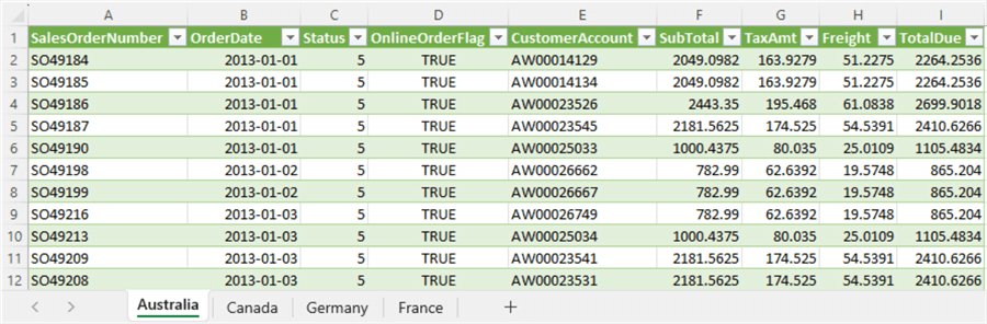
Figure 1 Sample data in the working file

In this exercise, we use Microsoft Excel for Microsoft 365 MSO (Version 2303 Build 16.0.16227.20202) 32-bit. While walking through the process of combining data from multiple spreadsheets in the same workbook into one single spreadsheet, we explore the following techniques:

Importing data from multiple spreadsheets into a workbook
Creating connections to spreadsheets
Creating a connection to a workbook
Creating a blank query
Appending queries as a new query
Organizing queries into query groups
Viewing query dependencies
Adding custom columns
Removing columns
Renaming columns
Replacing values in a column
Filtering queries
Viewing and modifying M code
Expanding structured columns
Duplicating an Excel worksheet

1 – Using the Append Queries as New Command to Combine Data in Multiple Worksheets

Power Query allows us to combine multiple queries into a single result. Using this feature, we can integrate data from different sources. This exercise combines data from several spreadsheets into a workbook. The technique also works for other sources, for example, CSV files and database tables. For simplicity, we assume all data has already been stored in Excel tables. We recommend using the Append Queries as New command to create a new query with the combined result. In this case, the original queries remain unaffected so that we can easily edit and debug the building blocks of the integrated query (Raviv, 2018).

1.1 Create Connections to the Worksheets

Open a new Excel workbook and go to the Data tab. Next, select the Data -> Get Data -> From File -> From Excel Workbook command to open the Import Data dialog box. Then, select workingfile.xlsx, as shown in Figure 2.

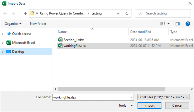
Figure 2 The Import Data dialog

Click on the Import button to open the Navigator dialog box. Then, select the Select multiple items checkbox. This way, we can choose various Excel tables, as shown in Figure 3. The right pane allows us to preview the data and inspect column headings. All tables should be in the same format. The spreadsheets are also available for selection; however, we prefer Excel tables. We convert the data into an Excel table to make a workbook act as a database. Cheusheva introduces three methods to create an Excel table and the ten most useful features of Excel tables (Cheusheva, 2023).

Figure 3 Select multiple Excel tables

Click on the Transform Data button to open the Power Query Editor. In the Combine group on the Home tab, we can find the Append Queries as New command, as shown in Figure 4.

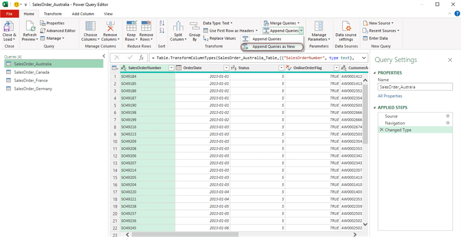
Figure 4 The Power Query Editor

1.2 Append Queries as a New Query

Select any query in the Queries pane, then select the Append Queries as New command. The Append dialog box appears. We choose the Three or more tables option and then add all tables to the Tables to append list box, as shown in Figure 5.

Figure 5 The Append dialog

Click the OK button to create a new query combining the four queries. The default name of the new query is Append1. The Query Settings pane allows us to change the query name. As shown in Figure 6, we give the query a meaningful name: SalesOrder.

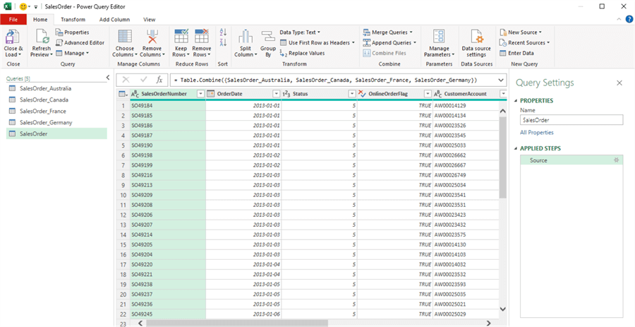
Figure 6 Combine queries to a new query

1.3 Organize Queries into Groups

There are five queries in the Queries pane. To help people easily understand and edit these queries, we organize them into different groups. We can group them based on content, functionality, or other criteria. In this exercise, we generate reports from the combined query. Therefore, we can put all four other queries into a group. We named the group "Import Data." This way, we do not need to check queries in this folder if performing data manipulation.

To create a new query group, right-click the empty area in the Queries pane to open the context menu, as shown in Figure 7.

Figure 7 The context menu from the Queries pane

Select the New Group… option from the context menu to open the New Group dialog box. Then, give the group a name, as shown in Figure 8.

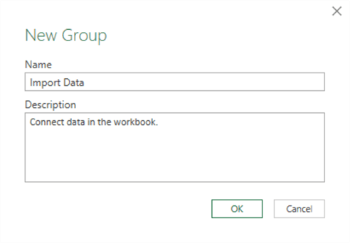
Figure 8 The New Group dialog

Click the OK button to create the group. Next, right-click on the query "SalesOrder_Australia" in the Queries pane to open the context menu. Then, select the newly formed group (i.e., the Import Data group) under the Move To Group menu item, as shown in Figure 9, to move the query to the group.

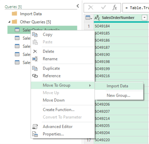
Figure 9 Move queries to the group

Use the same method to move SalesOrder_Canada, SalesOrder_France, and SalesOrder_Germany queries to the "Import Data" group. The Queries pane should look like Figure 10.

Figure 10 Add queries to the query group

1.4 Add New Columns to the Connection Queries

We want to add a new "Territory" column to each query to distinguish the sales orders. We can find the value of the new "Territory" column from the query name. For example, all sales orders in the SalesOrder_Australia query should belong to the Australia territory. We will edit all queries in the Import Data group to tag all sales orders with a territory.

Select the SalesOrder_Australia query in the Queries pane. Click the Add Column -> Custom Column button in the Ribbon to open the Custom Column dialog box. As shown in Figure 11, we name the new column Territory and define the formula as follows:

="Australia"

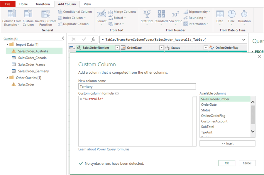
Figure 11 Add a new column

Click OK to close the dialog box and add the new column to the SalesOrder_Australia query. We repeat the process and add the new column to the other three queries in the Import Data group. We then select the SalesOrder query to preview the data. The combined query automatically includes the new column in the appended query. As shown in Figure 12, we tag each sales order with a territory.

Figure 12 Tag the sales orders with a new column

1.5 View Query Dependencies

We imported data from spreadsheets into Power Queries and created four connection queries. We then combined all these queries into a new query. We can use the View -> Query Dependencies command to show the relationships between these queries. When the data preparation contains complex transformations, the relationships help us understand and maintain these queries.

Open the View tab. Next, click the Query Dependencies button in the Dependencies group to open the Query Dependencies dialog box, as shown in Figure 13.

Figure 13 Query dependencies

1.6 Load the Combined Query into a Worksheet

We combined data from four Excel tables into the query "SalesOrder." We can perform further data transformation on this query, add the query to a data model, or create reports based on this query. For demonstration purposes, we load data into a worksheet.

Select the Close & Load -> Close & Load To… command in the Close group on the Home tab. The Import Data dialog box appears as shown in Figure 14. Then, select the Only Create Connection option in the dialog box.

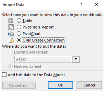
Figure 14 The Import Data dialog

Click on the OK button to close the Power Query Editor. In the Excel interface, select the Data -> Queries & Connections command to display the Queries & Connections pane on the right of the Excel interface. We can see all queries created in the Power Query Editor. Right-click on the query "SalesOrder" and select the Load To… command in the context menu, as shown in Figure 15.

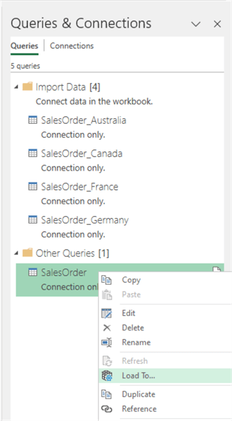
Figure 15 Load the query result to a worksheet

The Import Data dialog box appears as shown in Figure 16. Select the Table and Existing worksheet options in the dialog box.

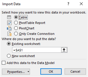
Figure 16 Load the data to an Excel table

Click the OK button to close the dialog box and load the data into a worksheet, as shown in Figure 17. We rename the worksheet "SalesOrder." When there is any change in the Excel tables, we can click the "Data -> Refresh All" button in the Ribbon to reload the data.

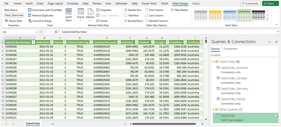
Figure 17 The worksheet with combined data

2 – Using a Robust Method to Detect New Worksheets

We explored combining data from multiple worksheets into a new worksheet. We first created four queries to import four Excel tables, respectively. We then combined the queries into a new query. The process is simple and understandable. However, when adding a new worksheet that contains data in a new sales territory, we must modify the process to add the new Excel table. Therefore, when the workbook may have new worksheets, we need a robust method to automatically create connections to the new sheets.

2.1 Create a Connection to the Excel Workbook

We first open a new Excel workbook, following the steps described in Section 1.1. Then go to the Data tab and select the Get Data -> From File -> From Excel Workbook command to open the Import Data dialog box. Next, select workingfile.xlsx. After clicking on the Import button, the Navigator dialog box appears. Rather than picking individual Excel tables, we choose the workbook, as shown in Figure 18.

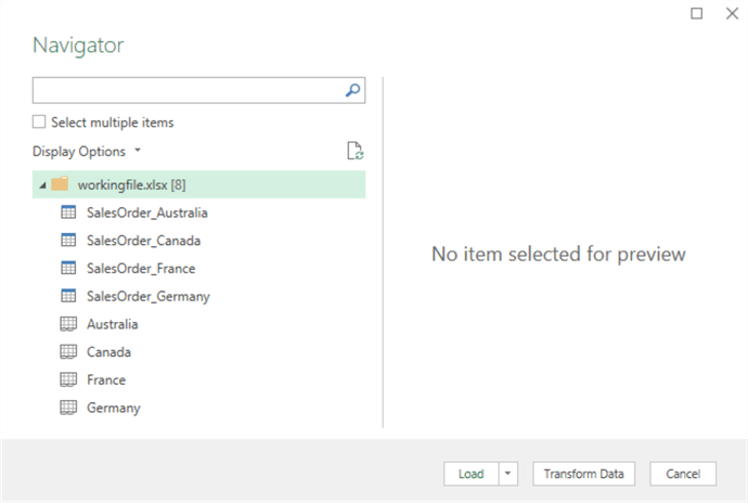
Figure 18 Select the workbook in the Navigator dialog

Click on the Transform Data button to open the Power Query Editor. We preview the contents of the workbook, as shown in Figure 19.

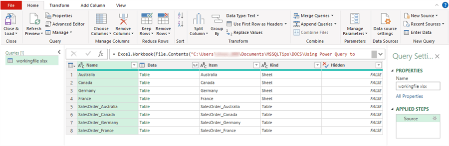
Figure 19 Preview the contents on the workbook

2.2 Add a Filter to the Query to Select Excel Tables

We only want to combine data in Excel tables. Click on the inverted triangle beside the Kind column heading to open the column header drop-down. Then, we select the Table option, as shown in Figure 20.

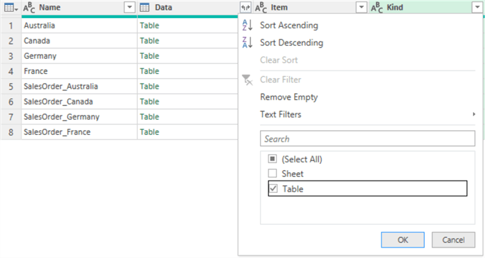
Figure 20 Add a filter to a text column

Click on the OK button to confirm the settings. We can check the M formula in the formula bar, as shown in Figure 21.

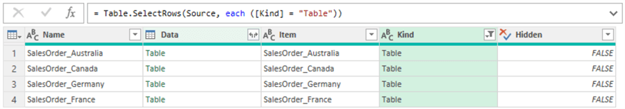
The M formular to filter values in a column

Figure 21 The M formula to filter values in a column

Sometimes, editing data transformations by modifying the M formula is convenient. For example, the following formula selects all rows whose [Kind] column has a value of "Table" and whose [Hidden] column has a value of false.

= Table.SelectRows(Source, each [Kind] = "Table" and [Hidden] = false)

2.3 Remove Unnecessary Columns

We only need the Name and Data columns; therefore, we want to remove the Item, Kind, and Hidden columns. Press and hold the CTRL key, then click on the headings of unneeded columns to select them. Next, select the Home -> Remove Columns command. The preview of the query result should look like Figure 22.

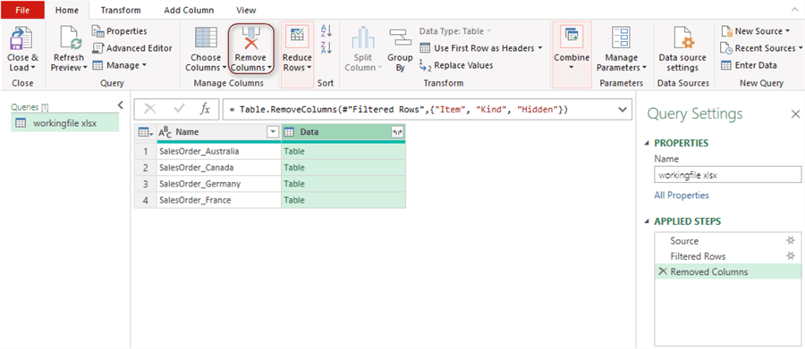
Figure 22 Remove unneeded columns

2.4 Rename Columns

Select the Name column, and then select the Transform -> Rename command. The column heading becomes editable. Next, change the header to "Territory" and press Enter to confirm the change. Figure 23 illustrates the method.

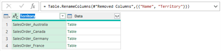
Figure 23 Rename a column

We modify the formula in the formula bar to change the Data column heading. We can copy the following M code to the formula bar. The preview of the query result should look like Figure 24.

= Table.RenameColumns(#"Removed Columns",{{"Name", "Territory"},{"Data", "Content"}})

Figure 24 Use the formula bar to rename columns

2.5 Replace Values in a Column

The Territory column contains the query names. We can extract territory names from the query names by removing the "SalesOrder_" prefix. We first select the Territory column. Then select the Transform -> Replace Values -> Replace Values command to open the Replace Values dialog box. As shown in Figure 25, we replace the value "SalesOrder_" with an empty value.

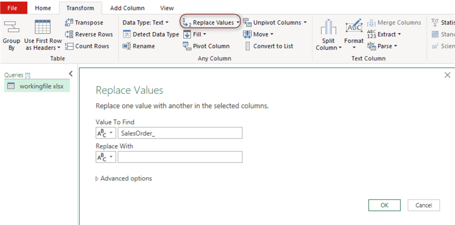
Figure 25 The Replace Values dialog box

Click on the OK button to confirm the transformation. Figure 26 shows the preview of the query result.

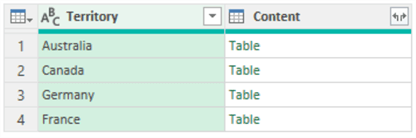
Figure 26 Extract territory names from the query names

2.6 Expand a Table-Structured Column.

The Content column is a table-structured column that stores a table. Each table value contains data from a corresponding Excel table. We can select a cell to preview the table’s contents at the bottom of the dialog box, as shown in Figure 27.

Figure 27 Preview a cell in the table-structured column

Click the expand icon beside the Content column heading to open the column name list box, as shown in Figure 28. Then, uncheck the Use original column name as prefix checkbox.

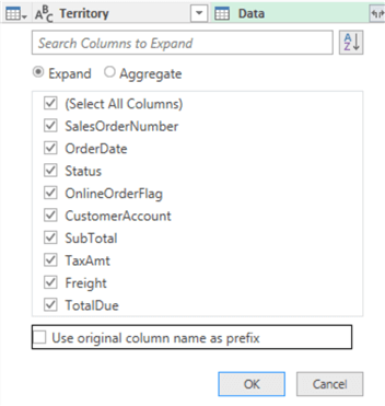
Figure 28 Expand a table-structured column

Next, click on the OK button to expand the table column. Figure 29 shows a preview of the combined query result.

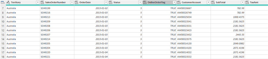
Figure 29 Preview the result of combined query

2.7 Load a Combined Query into the Worksheet

We have integrated four Excel tables into one query called "workingfile.xlsx." We may need other transformations to reshape the data. If so, we can add more transformation steps to the query. However, we load data into a worksheet for demonstration purposes in this exercise.

Click the Close & Load button in the Close group on the Home tab to load the data into a new worksheet. The new worksheet has the same name as the query name (i.e., workingfile.xlsx). The interface of the workbook should look like Figure 30.

Figure 30 The sample data in the new worksheet

2.8 Update and Refresh the Data

In everyday business operations, users add sales orders to the workbook. When creating a new sales territory, they must add a new worksheet to the workbook to record the sales transactions. We want to confirm that the combined query should automatically connect the data in the new worksheet.

First, we check the data before adding the new sheet. Click on the inverted triangle beside the Territory column to view the distinct values in this column, as shown in Figure 31.

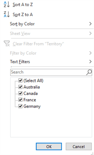
Figure 31 Distinct values in the Territory column

Then, we create a fake worksheet for testing purposes. Open the workingfile.xlsx file to access four worksheets, as shown in Figure 1. Then, hold the CTRL key. Next, click and drag the France sheet to the right. When releasing the mouse button, we create a copy of the France sheet. Name the new sheet, Mexico. We then change the Excel table name to SalesOder_Mexico, as shown in Figure 32.

Figure 32 Add a new worksheet to the workbook

Save and close the working file. Then, activate the workbook with the combined query and click the Data -> Refresh All button. Next, click on the inverted triangle beside the Territory column again. The column header drop-down appears, as shown in Figure 33. The column contains the value "Mexico," which indicates that the combined query imported data from the new worksheet.

Figure 33 The combined query automatically connects data in the new worksheet

3 – Combining Data from Multiple Worksheets into a New Worksheet

We imported data from multiple spreadsheets into a new workbook. However, we may need to create a master view in the same workbook where the transactional data lives. The Power Query M formula language provides a function to return the contents of the current Excel workbook:

= Excel.CurrentWorkbook()

The formula returns tables, named ranges, and dynamic arrays but does not return sheets. Therefore, we should put data in Excel tables to use this formula.

3.1 Create a Blank Query

Open the downloaded workbook (i.e., workingfile.xlsx), which should look like Figure 1. Click on the Data -> Get Data -> From Other Sources -> Blank Query command, as shown in Figure 34, to open the Power Query Editor.

Figure 34 The Blank Query command

By default, the name of the blank query is Query1. We rename the query MasterView via the Query Settings pane. Then, type the following formula in the formula bar:

=Excel.CurrentWorkbook()

After hitting the Enter key, we can preview the result of the function, as shown in Figure 35. The result shows a list of all detected Excel tables in the workbook. Note that M code is case-sensitive, so we must type the text exactly as shown above.

Figure 35 Excel tables in the current workbook

3.2 Add a Filter to the Query to Avoid Recursion

The formula =Excel.CurrentWorkbook() gives us a list of Excel tables in the current workbook. When we add new Excel tables to the workbook, the formula can detect these tables. This feature helps create a robust solution to combine Excel tables. However, the drawback is that the combined data may include unexpected data. Especially when we add a new worksheet with the combined data, the combined query sources its own results (Gharani, 2020). Therefore, we must ensure that we combine only those tables we want to combine. In this exercise, we want to filter the query to only include tables whose table names begin with "SalesOrder_."

Expand the Name column filter control, as shown in Figure 36.

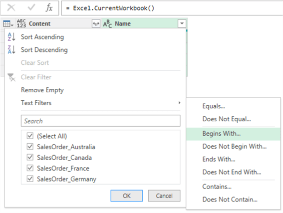
Figure 36 The Name column filter control

Select the Text Filters -> Begins With… command to open the Filter Rows dialog box. We configure the settings according to Figure 37. Click the OK button to confirm the settings. This transformation step does not change the query result at this moment. However, the filter can select only sales transaction data for combination and prevent recursion.

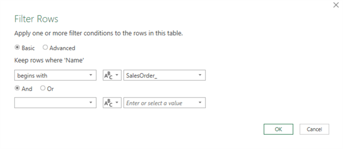
Figure 37 The Filter Rows dialog

3.3 Use Power Query to Transform Data

The query result shown in Figure 35 is the same as in Figure 24, except for the column order. Therefore, we can follow the steps from Section 2.5 to Section 2.8 to transform data, load data into a new worksheet, and conduct a refreshing data test. Figure 38 shows the test result.

Figure 38 Add a master view to the current workbook

If we do not add a filter in Section 3.2, the MasterView query will load data from the MasterView worksheet. Therefore, recursion occurs, and the combined query can not provide accurate data.

Summary

We often combine the same formatted data from several worksheets into a new sheet to obtain an overview of the data. The article explored three methods that can address different business requirements.

The first method created connection queries to the data in each worksheet and then combined all the connection queries. To make the combined query automatically include data in a new worksheet, we introduced a robust method that created a connection query to the workbook. The third method established a connection to the current workbook. This way, the workbook could provide an overview of the raw data.

We also covered some practical techniques, for example, organizing queries into groups, viewing query dependencies, replacing values in a column, and expanding a table-structure column.

Reference

Bansal, S. (2018). Combine Data From Multiple Worksheets into a Single Worksheet in Excel. https://trumpexcel.com/combine-multiple-worksheets/

Cheusheva, S. (2023). Excel table: end-to-end tutorial with examples. https://www.ablebits.com/office-addins-blog/excel-table-tutorial/.

Gharani, L. (2020). How to Combine Excel Sheets with Power Query. https://www.xelplus.com/combine-excel-sheets-power-query/.

Kenyon, M. (2022). How to Create a Searchable Database in Excel. https://www.skuvault.com/blog/how-to-create-a-searchable-database-in-excel/.

Raviv, G. (2018). Collect, Combine, and Transform Data Using Power Query in Excel and Power BI, First Edition.

Next Steps

Understanding how to use Power Query, a potent tool for data manipulation, is worthwhile. With Power Query, business users can explore databases and perform data transformations without the help of IT. We use the Power Query Editor to develop and maintain queries. The editor converts each step into Power Query M code. We do not need to memorize all these commands and M code functions. Instead, we should practice transforming data for reporting purposes and understand the reasons behind the scenes. We can learn something better and faster if we practice it. In addition, we need to develop skills that translate business questions to data questions, then use data to answer data questions and, therefore, address the business questions.
Check out these related tips:

About the author

Nai Biao Zhou is a Senior Software Developer with 20+ years of experience in software development, specializing in Data Warehousing, Business Intelligence, Data Mining and solution architecture design.

This author pledges the content of this article is based on professional experience and not AI generated.

View all my tips

Article Last Updated: 2023-07-18

Using Power Query to Combine Data from Multiple Sheets in Excel