Problem
In this article, we look at an ensemble AI model which can be considered a collection of two or more AI models that complement each other to arrive at an outcome for a set of historical data.
Solution
A good place to start is by appreciating the basics of an AI model. An AI model takes data as input and simulates a decision-making process to arrive at an outcome, such as dates and prices for buying and/or selling a security, assessing how much and when to replenish in-stock inventory items, or predicting temperature and rainfall observations from a weather station for tomorrow, next week, or next month. A SQL Server professional can think of an AI model as a set of one or more queries that return some results sets. The query statements and their results sets are meant to match or exceed the performance of an expert human decision-maker.
As a SQL Server professional, you can think of the data for an AI model as the data inside a SQL Server instance (or data that you can import to SQL Server from an online data source). Processing steps are implemented as successive queries that pass results sets from one query to the next through the final processing step in the AI model. The final results set is the implemented version of the AI model. With time series data, which are the focus of the models in this tip, an AI model can run repetitively until there are no remaining historical data to evaluate the model.
An ensemble AI model can be considered a collection of two or more AI models that complement each other to arrive at an outcome for a set of historical data. Each model in an AI ensemble model should have its own distinct set of rules. Additionally, each model in an ensemble AI model needs to have specific rules for combining its results sets with the results sets for one or more other elements in an ensemble model. The combined results sets from the ensemble model elements is the ensemble model.
The solution code for the problem statement includes demonstrations of how to apply standard T-SQL coding techniques for AI applications. Among the standard T-SQL coding techniques for AI modeling covered in this tip are:
- Creating fresh tables with drop table if exists and select into statements
- Creating and invoking stored procedures
- Syntax examples for lag and lead functions as well as min and max functions
- Complementary applications for local temp tables, global temp tables, and table variables
- Reconfiguring a normalized results set as a de-normalized results set to speed code execution
An Overview of the Ensemble Model for this Tip
The data for this tip processes security price data for six tickers. The six tickers are for three pairs of ETF securities based on three major market indexes. The indexes are the Dow Industrial Average, S&P 500, and Nasdaq 100. One member of each pair of securities (DIA, QQQ, SPY) aims to follow the price performance of its underlying index on a proportional basis for each trading day. The other member of each pair of securities (UDOW, TQQQ, SPXL) aims to have its price performance remain in a three-to-one relation to its underlying index on a daily trading day basis. A prior tip titled “SQL Server Data Mining for Leveraged Versus Unleveraged ETFs as a Long-Term Investment” demonstrated how to collect and save historical price and volume data from Yahoo Finance for these six tickers to a SQL Server table named DataScience.dbo.symbol_date.
The download from the prior tip includes the original CSV files from Yahoo Finance and the T-SQL code for transferring the file contents to the DataScience.dbo.symbol_date table. The next two screenshots show the first and last eight rows from the table. There is one row for each trading day on which a ticker symbol trades. Across all six tickers starting from each ticker’s initial public offering date through November 30, 2022, there are a maximum of 29731 rows of data.


There are two AI model elements in the ensemble AI model for this tip:
- The first AI model is called the “close_gt_ema_10_model”. This model designates a date on which to buy a security whenever the close value for the preceding two trading days is greater than the exponential moving average with a period length of 10, which is also preceded by another two trading days in which the close value is not greater than the exponential moving average with a period length of 10. The model ends the hold period for a security ten days after it is bought.
- The second AI model is called the “seasonal_include_model”. This model treats each month as a season of the year for computing a seasonal factor over a timeframe. The T-SQL code for computing these monthly seasonal factors is described in the “Computing seasonality factors by month across year” section of this prior tip.
The rule for combining the two models are as follows.
- Use the close_gt_ema_10_model to pick an initial set of buy dates for each of the six ticker symbols
- Then, use the seasonal_include_model to identify months for a symbol that are most likely to result in winning trades
- Finally, only include buy dates from the close_gt_ema_10_model where the buy dates belong to a month that is from the top half of months based on the seasonal_include_model. Exclude buy dates from the close_gt_ema_10_model that are not from the top half of months based on the seasonal_include_model. It is this last combining rule that makes the model from this tip an ensemble AI model – that is, the ensemble AI model is like a medley from both the close_gt_ema_10_model and the seasonal_include_model.
Implementing the close_gt_ema_10_model
The implementation of the close_gt_ema_10_model requires a dataset derived from the symbol_date table. The three essential columns from this table are the symbol ticker column for one of the six tickers for which data are available from the table, the close value column for each ticker on a trading date, and the close date value column for each ticker symbol which start with the initial public offering date for a ticker through the last date for which data was collected for implementing the model. The initial public offering date is the first date for which shares of a security are available for trading. Data collection for all six tickers ceased on November 30, 2022.
In addition to the preceding three underlying source data columns, several other columns need to be calculated. Many of these calculated columns depend directly on the exponential moving average with a period length of 10 for the close value of the current trading date (ema_10). If you are not already familiar with exponential moving averages, you may find either or both of these two prior tips informative:
- An earlier article titled “Exponential Moving Average Calculation in SQL Server” briefly introduces exponential moving averages and how to calculate them for a dataset already in SQL Server.
- A recent article titled “Adding a Buy-Sell Model to a Buy-and-Hold Model with T-SQL” provides an example of computing exponential moving averages with the same underlying data source as the one used in this tip. This second article can provide an additional resource to help you understand this tip and build your capability to create AI models in SQL Server.
As with many AI models, the evaluation of the close_gt_ema_10_model requires looking back over preceding periods to the current one.
- The close_gt_ema_10_model compares the close value and the ema_10 values for each of the prior four periods. These previous four periods (trading days) are examined to determine if the close values are rising relative to the ema_10 values
- If an uptrend of the close values relative to ema_10 values is detected, then the model specifies a buy date for the current trading date and a sell date for 10 days after the current trading date
- If the close value for 10 days after the current trading date is greater than the current trading date, then the model has a winning buy/sell cycle
The following create procedure statement is the most recent version of my T-SQL code for computing exponential moving average values for a column of historical time series values, such as the close values in this tip. This version of the stored procedure takes advantage of decimal(19,4) for storing and processing monetary data type values.
- The stored procedure operates on close values originating in the symbol_date table; the ema values output by the stored procedure are saved in #temp_for_ema
- Three parameters adjust the performance of the stored procedure
- The @symbol parameter designates the ticker symbol for which to compute ema values
- The @period parameter indicates the period length of the ema values
- The @alpha parameter is the weighting value for the close value for the current period, and (1-@alpha) is the weighting value for the ema for the prior period
Use DataScience
go

drop procedure if exists [dbo].[usp_ema_computer_with_dec_vals]
go

create procedure [dbo].[usp_ema_computer_with_dec_vals]
   -- Add the parameters for the stored procedure here
    @symbol nvarchar(10)  -- for example, assign as 'SPY'
   ,@period dec(19,4)     -- for example, assign as 12
   ,@alpha dec(14,4)      -- for example, assign as 2/(12 + 1)
as

begin
   -- suppress row counts for output from usp
   set nocount on;

   -- parameters to the script are
   -- @symbol identifier for set of time series values
   -- @period number of periods for ema
   -- @alpha weight for current row time series value

   -- initially populate #temp_for_ema for ema calculations
   -- @ema_first is the seed
   declare @ema_first dec(19,4) =
   (select top 1 [close] from [dbo].[symbol_date] where symbol = @symbol order by [date])

   -- create base table for ema calculations

   drop table if exists #temp_for_ema

   -- ema seed run to populate #temp_for_ema
   -- all rows have first close price for ema
   select
    [date]
   ,[symbol]
   ,[close]
   ,row_number() OVER (ORDER BY [Date]) [row_number]
   ,@ema_first ema
   into #temp_for_ema
   from [dbo].[symbol_date]
   where symbol = @symbol
   order by row_number

   -- NULL ema values for first period
   update #temp_for_ema
   set
   ema = NULL
   where row_number = 1

   -- calculate ema for all dates in time series
   -- @alpha is the exponential weight for the ema
   -- start calculations with the 3rd period value
   -- seed is close from 1st period; it is used as ema for 2nd period

   -- set @max_row_number int and initial @current_row_number
   -- declare @today_ema
   declare @max_row_number int = (select max(row_number) from #temp_for_ema)
   declare @current_row_number int = 3
   declare @today_ema dec(19,4)

   -- loop for computing successive ema values
   while @current_row_number <= @max_row_number
   begin

    set @today_ema =
    (
    -- compute ema for @current_row_number
    select
    top 1
    ([close] * @alpha) + (lag(ema,1) over (order by [date]) * (1 - @alpha)) ema_today

    from #temp_for_ema
    where row_number >=  @current_row_number -1 and row_number <= @current_row_number
    order by row_number desc
    )

    -- update current row in #temp_for_ema with @today_ema
    -- and increment @current_row_number
    update #temp_for_ema
    set
     ema = @today_ema
    where row_number = @current_row_number

    set @current_row_number = @current_row_number + 1

   end

   -- display the results set with the calculated values
   -- on a daily basis
   select
    date
   ,symbol
   ,[close]
   ,@period period_length
   ,ema ema
   from #temp_for_ema
   where row_number < = @max_row_number
   order by row_number

end
go
Here is a script excerpt for invoking the usp_ema_computer_with_dec_vals stored procedure created in the preceding create procedure statement. The script repeatedly invokes the stored procedure for the six tickers examined in this tip. Results are stored in the ema_period_symbol_with_dec_vals table via an insert into statement. In addition to computing ema_10 values for close values, the code also computes ema_30, ema_50, and ema_200 for close values. This was convenient because the original code for invoking the usp_ema_computer_with_dec_vals stored procedure was excerpted from another application that required exponential moving averages with period lengths of 10, 30, 50, and 200.
use DataScience
go


-- create a fresh copy of the [dbo].[ema_period_symbol_with_dec_vals] table

drop table if exists dbo.ema_period_symbol_with_dec_vals

create table [dbo].[ema_period_symbol_with_dec_vals](
   [date] [date] NOT NULL,
   [symbol] [nvarchar](10) NOT NULL,
   [close] [decimal](19, 4) NULL,
   [period_length] [int] NOT NULL,
   [ema] [decimal](19, 4) NULL,
primary key clustered
(
   [symbol] ASC,
   [date] ASC,
   [period_length] ASC
)WITH (PAD_INDEX = OFF, STATISTICS_NORECOMPUTE = OFF, IGNORE_DUP_KEY = OFF, ALLOW_ROW_LOCKS = ON, ALLOW_PAGE_LOCKS = ON, OPTIMIZE_FOR_SEQUENTIAL_KEY = OFF) ON [PRIMARY]
) ON [PRIMARY]
go


-- populate a fresh copy of ema_period_symbol_with_dec_vals
-- with the [dbo].[ema_period_symbol_with_dec_vals] stored proc
-- based on four period lengths (10, 30, 50, 200)
-- for six symbols (SPY, SPXL, QQQ, TQQQ, DIA, UDOW)


-- populate 10, 30, 50, 200 period_length emas for SPY ticker
insert into [dbo].[ema_period_symbol_with_dec_vals]
exec [dbo].[usp_ema_computer_with_dec_vals] 'SPY', 10, .1818
insert into [dbo].[ema_period_symbol_with_dec_vals]
exec [dbo].[usp_ema_computer_with_dec_vals] 'SPY', 30, .0645
insert into [dbo].[ema_period_symbol_with_dec_vals]
exec [dbo].[usp_ema_computer_with_dec_vals] 'SPY', 50, .0392
insert into [dbo].[ema_period_symbol_with_dec_vals]
exec [dbo].[usp_ema_computer_with_dec_vals] 'SPY', 200, .0100

-- populate 10, 30, 50, 200 period_length emas for SPXL ticker
insert into [dbo].[ema_period_symbol_with_dec_vals]
exec [dbo].[usp_ema_computer_with_dec_vals] 'SPXL', 10, .1818
insert into [dbo].[ema_period_symbol_with_dec_vals]
exec [dbo].[usp_ema_computer_with_dec_vals] 'SPXL', 30, .0645
insert into [dbo].[ema_period_symbol_with_dec_vals]
exec [dbo].[usp_ema_computer_with_dec_vals] 'SPXL', 50, .0392
insert into [dbo].[ema_period_symbol_with_dec_vals]
exec [dbo].[usp_ema_computer_with_dec_vals] 'SPXL', 200, .0100

-- populate 10, 30, 50, 200 period_length emas for QQQ ticker
insert into [dbo].[ema_period_symbol_with_dec_vals]
exec [dbo].[usp_ema_computer_with_dec_vals] 'QQQ', 10, .1818
insert into [dbo].[ema_period_symbol_with_dec_vals]
exec [dbo].[usp_ema_computer_with_dec_vals] 'QQQ', 30, .0645
insert into [dbo].[ema_period_symbol_with_dec_vals]
exec [dbo].[usp_ema_computer_with_dec_vals] 'QQQ', 50, .0392
insert into [dbo].[ema_period_symbol_with_dec_vals]
exec [dbo].[usp_ema_computer_with_dec_vals] 'QQQ', 200, .0100

-- populate 10, 30, 50, 200 period_length emas for TQQQ ticker
insert into [dbo].[ema_period_symbol_with_dec_vals]
exec [dbo].[usp_ema_computer_with_dec_vals] 'TQQQ', 10, .1818
insert into [dbo].[ema_period_symbol_with_dec_vals]
exec [dbo].[usp_ema_computer_with_dec_vals] 'TQQQ', 30, .0645
insert into [dbo].[ema_period_symbol_with_dec_vals]
exec [dbo].[usp_ema_computer_with_dec_vals] 'TQQQ', 50, .0392
insert into [dbo].[ema_period_symbol_with_dec_vals]
exec [dbo].[usp_ema_computer_with_dec_vals] 'TQQQ', 200, .0100

-- populate 10, 30, 50, 200 period_length emas for DIA ticker
insert into [dbo].[ema_period_symbol_with_dec_vals]
exec [dbo].[usp_ema_computer_with_dec_vals] 'DIA', 10, .1818
insert into [dbo].[ema_period_symbol_with_dec_vals]
exec [dbo].[usp_ema_computer_with_dec_vals] 'DIA', 30, .0645
insert into [dbo].[ema_period_symbol_with_dec_vals]
exec [dbo].[usp_ema_computer_with_dec_vals] 'DIA', 50, .0392
insert into [dbo].[ema_period_symbol_with_dec_vals]
exec [dbo].[usp_ema_computer_with_dec_vals] 'DIA', 200, .0100

-- populate 10, 30, 50, 200 period_length emas for UDOW ticker
insert into [dbo].[ema_period_symbol_with_dec_vals]
exec [dbo].[usp_ema_computer_with_dec_vals] 'UDOW', 10, .1818
insert into [dbo].[ema_period_symbol_with_dec_vals]
exec [dbo].[usp_ema_computer_with_dec_vals] 'UDOW', 30, .0645
insert into [dbo].[ema_period_symbol_with_dec_vals]
exec [dbo].[usp_ema_computer_with_dec_vals] 'UDOW', 50, .0392
insert into [dbo].[ema_period_symbol_with_dec_vals]
exec [dbo].[usp_ema_computer_with_dec_vals] 'UDOW', 200, .0100
The ema_period_symbol_with_dec_vals table returns values in a normalized format, which is common for relational databases, but this format can be an inefficient way of storing time series data. The normalized format can be transformed to another format that is more efficient for storing and retrieving time series data. For example, the following script reconfigures the contents of the ema_period_symbol_with_dec_vals table into a new table named close_and_emas. The number of rows in the ema_period_symbol_with_dec_vals table is 118924, but when the data are reconfigured in the more efficient format of the close_and_emas table, the number of rows shrinks to 29731.
use DataScience
go

-- join and concatenate rows
-- for symbols and period_lengths
-- count of rows in outer query is 29731

drop table if exists dbo.close_and_emas

select *
into dbo.close_and_emas
from
(
select *
from
(
select
 for_ema_10.symbol
,for_ema_10.date
,for_ema_10.[close]
,for_ema_10.ema_10
,for_ema_30.ema_30
,for_ema_50.ema_50
,for_ema_200.ema_200
from
(
select
 symbol
,date
,[close]
,period_length
,ema [ema_10]
from ema_period_symbol_with_dec_vals
where symbol = 'SPY' and period_length = 10
) for_ema_10

join

(
select
 symbol
,date
--,[close]
--,period_length
,ema [ema_30]
from ema_period_symbol_with_dec_vals
where symbol = 'SPY' and period_length = 30
) for_ema_30

 on for_ema_10.symbol = for_ema_30.symbol and
    for_ema_10.[date] = for_ema_30.[date]

join

(
select
 symbol
,date
--,[close]
--,period_length
,ema [ema_50]
from ema_period_symbol_with_dec_vals
where symbol = 'SPY' and period_length = 50
) for_ema_50

 on for_ema_10.symbol = for_ema_50.symbol and
    for_ema_10.[date] = for_ema_50.[date]

join

(
select
 symbol
,date
--,[close]
--,period_length
,ema [ema_200]
from ema_period_symbol_with_dec_vals
where symbol = 'SPY' and period_length = 200
) for_ema_200

 on for_ema_10.symbol = for_ema_200.symbol and
    for_ema_10.[date] = for_ema_200.[date]
) for_SPY

union

select *
from
(
select
 for_ema_10.symbol
,for_ema_10.date
,for_ema_10.[close]
,for_ema_10.ema_10
,for_ema_30.ema_30
,for_ema_50.ema_50
,for_ema_200.ema_200
from
(
select
 symbol
,date
,[close]
,period_length
,ema [ema_10]
from ema_period_symbol_with_dec_vals
where symbol = 'SPXL' and period_length = 10
) for_ema_10

join

(
select
 symbol
,date
--,[close]
--,period_length
,ema [ema_30]
from ema_period_symbol_with_dec_vals
where symbol = 'SPXL' and period_length = 30
) for_ema_30

 on for_ema_10.symbol = for_ema_30.symbol and
    for_ema_10.[date] = for_ema_30.[date]

join

(
select
 symbol
,date
--,[close]
--,period_length
,ema [ema_50]
from ema_period_symbol_with_dec_vals
where symbol = 'SPXL' and period_length = 50
) for_ema_50

 on for_ema_10.symbol = for_ema_50.symbol and
    for_ema_10.[date] = for_ema_50.[date]

join

(
select
 symbol
,date
--,[close]
--,period_length
,ema [ema_200]
from ema_period_symbol_with_dec_vals
where symbol = 'SPXL' and period_length = 200
) for_ema_200

 on for_ema_10.symbol = for_ema_200.symbol and
    for_ema_10.[date] = for_ema_200.[date]

) for_SPXL

Union

select *
from
(
select
 for_ema_10.symbol
,for_ema_10.date
,for_ema_10.[close]
,for_ema_10.ema_10
,for_ema_30.ema_30
,for_ema_50.ema_50
,for_ema_200.ema_200
from
(
select
 symbol
,date
,[close]
,period_length
,ema [ema_10]
from ema_period_symbol_with_dec_vals
where symbol = 'QQQ' and period_length = 10
) for_ema_10

join

(
select
 symbol
,date
--,[close]
--,period_length
,ema [ema_30]
from ema_period_symbol_with_dec_vals
where symbol = 'QQQ' and period_length = 30
) for_ema_30

 on for_ema_10.symbol = for_ema_30.symbol and
    for_ema_10.[date] = for_ema_30.[date]

join

(
select
 symbol
,date
--,[close]
--,period_length
,ema [ema_50]
from ema_period_symbol_with_dec_vals
where symbol = 'QQQ' and period_length = 50
) for_ema_50

 on for_ema_10.symbol = for_ema_50.symbol and
    for_ema_10.[date] = for_ema_50.[date]

join

(
select
 symbol
,date
--,[close]
--,period_length
,ema [ema_200]
from ema_period_symbol_with_dec_vals
where symbol = 'QQQ' and period_length = 200
) for_ema_200

 on for_ema_10.symbol = for_ema_200.symbol and
    for_ema_10.[date] = for_ema_200.[date]
) for_QQQ

union

select *
from
(
select
 for_ema_10.symbol
,for_ema_10.date
,for_ema_10.[close]
,for_ema_10.ema_10
,for_ema_30.ema_30
,for_ema_50.ema_50
,for_ema_200.ema_200
from
(
select
 symbol
,date
,[close]
,period_length
,ema [ema_10]
from ema_period_symbol_with_dec_vals
where symbol = 'TQQQ' and period_length = 10
) for_ema_10

join

(
select
 symbol
,date
--,[close]
--,period_length
,ema [ema_30]
from ema_period_symbol_with_dec_vals
where symbol = 'TQQQ' and period_length = 30
) for_ema_30

 on for_ema_10.symbol = for_ema_30.symbol and
    for_ema_10.[date] = for_ema_30.[date]

join

(
select
 symbol
,date
--,[close]
--,period_length
,ema [ema_50]
from ema_period_symbol_with_dec_vals
where symbol = 'TQQQ' and period_length = 50
) for_ema_50

 on for_ema_10.symbol = for_ema_50.symbol and
    for_ema_10.[date] = for_ema_50.[date]

join

(
select
 symbol
,date
--,[close]
--,period_length
,ema [ema_200]
from ema_period_symbol_with_dec_vals
where symbol = 'TQQQ' and period_length = 200
) for_ema_200

 on for_ema_10.symbol = for_ema_200.symbol and
    for_ema_10.[date] = for_ema_200.[date]

) for_TQQQ

union
select *
from
(
select
 for_ema_10.symbol
,for_ema_10.date
,for_ema_10.[close]
,for_ema_10.ema_10
,for_ema_30.ema_30
,for_ema_50.ema_50
,for_ema_200.ema_200
from
(
select
 symbol
,date
,[close]
,period_length
,ema [ema_10]
from ema_period_symbol_with_dec_vals
where symbol = 'DIA' and period_length = 10
) for_ema_10


join

(
select
 symbol
,date
--,[close]
--,period_length
,ema [ema_30]
from ema_period_symbol_with_dec_vals
where symbol = 'DIA' and period_length = 30
) for_ema_30

 on for_ema_10.symbol = for_ema_30.symbol and
    for_ema_10.[date] = for_ema_30.[date]


join

(
select
 symbol
,date
--,[close]
--,period_length
,ema [ema_50]
from ema_period_symbol_with_dec_vals
where symbol = 'DIA' and period_length = 50
) for_ema_50

 on for_ema_10.symbol = for_ema_50.symbol and
    for_ema_10.[date] = for_ema_50.[date]


join

(
select
 symbol
,date
--,[close]
--,period_length
,ema [ema_200]
from ema_period_symbol_with_dec_vals
where symbol = 'DIA' and period_length = 200
) for_ema_200

 on for_ema_10.symbol = for_ema_200.symbol and
    for_ema_10.[date] = for_ema_200.[date]

) for_DIA

union

select *
from
(
select
 for_ema_10.symbol
,for_ema_10.date
,for_ema_10.[close]
,for_ema_10.ema_10
,for_ema_30.ema_30
,for_ema_50.ema_50
,for_ema_200.ema_200
from
(
select
 symbol
,date
,[close]
,period_length
,ema [ema_10]
from ema_period_symbol_with_dec_vals
where symbol = 'UDOW' and period_length = 10
) for_ema_10


join

(
select
 symbol
,date
--,[close]
--,period_length
,ema [ema_30]
from ema_period_symbol_with_dec_vals
where symbol = 'UDOW' and period_length = 30
) for_ema_30

 on for_ema_10.symbol = for_ema_30.symbol and
    for_ema_10.[date] = for_ema_30.[date]


join

(
select
 symbol
,date
--,[close]
--,period_length
,ema [ema_50]
from ema_period_symbol_with_dec_vals
where symbol = 'UDOW' and period_length = 50
) for_ema_50

 on for_ema_10.symbol = for_ema_50.symbol and
    for_ema_10.[date] = for_ema_50.[date]


join

(
select
 symbol
,date
--,[close]
--,period_length
,ema [ema_200]
from ema_period_symbol_with_dec_vals
where symbol = 'UDOW' and period_length = 200
) for_ema_200

 on for_ema_10.symbol = for_ema_200.symbol and
    for_ema_10.[date] = for_ema_200.[date]

) for_UDOW
) for_SPY_SPXL_QQQ_TQQQ_DIA_UDOW
The next script excerpt relies on the close_and_emas table as a data source to populate the #temp_with_criteria_for_start_cycles table for exposing the criteria for buy and sell decisions based on the close_gt_ema_10_model rules. The script does not make any decisions, but it does expose the criteria on which buy and sell decisions are subsequently made.
- There are four columns that serve as the primary criteria for buy and sell decisions. These columns have names of start_lag_4, start_lag_3, start_lag_2, and start_lag_1
- When the values for start_lag_4 through start_lag_1 have values of 0, 0, 1,1, then close values are generally increasing over the preceding four trading days. The model assumes this is a good time to buy a security
- The model assumes that a good time to sell a security is at the tenth day past the preceding buy date. The model makes this assumption on the belief that the close value exceeding the ema_10 value is a relatively short-term predictor of future performance
- As indicated above, the #temp_with_criteria_for_start_cycles table does not actually make buy and sell decisions. Therefore, the #temp_with_criteria_for_start_cycles table has 29731 rows – one for each trading day across all six tickers in the symbol_date table
drop table if exists #temp_with_criteria_for_start_cycles

-- THIS CODE DISPLAYS THE CRITERIA FOR
-- START CYCLES FROM SOURCE DATA
-- evaluate start lag indicator
-- according to
-- (start_lag_4 and start_lag_3) = 0 and
-- (start_lag_2 and start_lag_1) = 1
select
 *
,case
   when close_lag_4 <= ema_10_lag_4 then 0
   else 1
end start_lag_4
,case
   when close_lag_3 <= ema_10_lag_3 then 0
   else 1
end start_lag_3
,case
   when close_lag_2 > ema_10_lag_2 then 1
   else 0
end start_lag_2
,case
   when close_lag_1 > ema_10_lag_1 then 1
   else 0
end start_lag_1
into #temp_with_criteria_for_start_cycles
from
(
-- extract base data, compute lags for ema_10 and close
-- as well as compute [close]_lead_10
select
 symbol
,date
,[close]
,ema_10
-- compute ema_10 lags
,lag(ema_10,4) over (partition by symbol order by date) ema_10_lag_4
,lag(ema_10,3) over (partition by symbol order by date) ema_10_lag_3
,lag(ema_10,2) over (partition by symbol order by date) ema_10_lag_2
,lag(ema_10,1) over (partition by symbol order by date) ema_10_lag_1
-- compute close lags
,lag([close],4) over (partition by symbol order by date) close_lag_4
,lag([close],3) over (partition by symbol order by date) close_lag_3
,lag([close],2) over (partition by symbol order by date) close_lag_2
,lag([close],1) over (partition by symbol order by date) close_lag_1
-- compute [close]_lead_10
,lead([close],10) over (partition by symbol order by date) close_lead_10
 from DataScience.dbo.close_and_emas
 ) for_start_lag_indicators

-- optionally display #temp_with_criteria_for_start_cycles
   select * from #temp_with_criteria_for_start_cycles
The next code segment reflects the buy dates and prices and the corresponding sell prices based on the sell criterion indicated in the preceding script. There are only 1297 rows in the result set from the script excerpt below. These rows are for the 1297 buy signal rows indicated by column values for start_lag_4, start_lag_3, start_lag_2, and start_lag_1 columns.
drop table if exists #temp_with_close_and_close_lead_10_for_each_start_cycle

-- THIS CODE EXTRACTS AND DISPLAYS THE
-- START CYCLES BASED ON START CYCLE CRITERIA

-- save symbol, date, [close], and close_lead_10
-- in #temp_with_close_and_close_lead_10_for_each_start_cycle
-- from #temp_with_criteria_for_start_cycles
select
 symbol
,date
,[close]
,close_lead_10
into #temp_with_close_and_close_lead_10_for_each_start_cycle
from #temp_with_criteria_for_start_cycles
where
 start_lag_4=0 and
 start_lag_3=0 and
 start_lag_2=1 and
 start_lag_1=1

-- optionally display #temp_with_close_and_close_lead_10_for_each_start_cycle_plus_duration_in_years
   select * from #temp_with_close_and_close_lead_10_for_each_start_cycle
The key metric for evaluating model performance in this tip is the compound annual growth rate. This metric represents the change in the value of an investment from the first day of an investment through the last day of an investment. The first and last day of an investment depends on when some resources were initially devoted to buying an investment and, correspondingly, the last time an investment in a security is sold.
- In the context of the current tip, the date of the first investment in a security is the close date for the first trade of a security.
- Also, the date of the last investment in a security ends on the tenth trading day after the last date during which a security is bought.
The following script shows how to compute the duration between the first investment in a ticker symbol through the last sell date for a security.
- The beginning date of an investment for a security is the min(date) value for the date column from symbol_date table for a security
- The ending date of an investment for a security is the max function value for the date column from the symbol_date table for a security
- The duration in years between the beginning date and ending date for a security in years is the datediff function value between beginning and ending dates in months divided by 12. The script below rounds the datediff function value to two places after the decimal point.
- The script saves its results set to a local temp table named #temp_with_close_and_close_lead_10_for_each_start_cycle_plus_duration_in_years.
The following script shows that the close_gt_ema_10_model makes no assumptions about carrying over the change in value from the preceding buy/sell cycle to the next buy/sell cycle. Instead, the model merely buys a single share of a stock at close value for the current start cycle. There are any number of possible assumptions to make about carrying over the change in value from the preceding buy/sell cycle (along with amounts) to the next buy/sell cycle. This tip leaves it to future investigations to evaluate the effectiveness of changes to the amount invested in a security from one buy/sell cycle to the next one.
-- create and populate #temp_with_close_and_close_lead_10_for_each_start_cycle_plus_duration_in_years

drop table if exists #temp_with_close_and_close_lead_10_for_each_start_cycle_plus_duration_in_years

select
 #temp_with_close_and_close_lead_10_for_each_start_cycle.*
,for_duration_in_years.duration_in_years
into #temp_with_close_and_close_lead_10_for_each_start_cycle_plus_duration_in_years
from #temp_with_close_and_close_lead_10_for_each_start_cycle
join
(
-- DISPLAY THE BEGINNING AND ENDING DATES BY TICKER FROM SOURCE DATA
-- divide difference in months by 12.0 and round quotient to 2 places
-- after the decimal to get duration_in_years to hundredths of a year
SELECT
    symbol
   ,min([Date]) [beginning date]
   ,max([Date]) [ending date]
   ,round((DATEDIFF(month, min([Date]), max([Date]))/12.0),2) duration_in_years
from [DataScience].[dbo].[symbol_date]
group by symbol
) for_duration_in_years
on #temp_with_close_and_close_lead_10_for_each_start_cycle.symbol = for_duration_in_years.symbol

order by
 #temp_with_close_and_close_lead_10_for_each_start_cycle.symbol
,#temp_with_close_and_close_lead_10_for_each_start_cycle.date
The next script excerpt saves a duplicate of the same results set as the one generated by the preceding script. The difference between the preceding script and the next script is that the following script saves its results set in a global temp table named ##temp_with_close_and_close_lead_10_for_each_start_cycle_plus_duration_in_years. The prior script excerpt saves its results set in a local temp table (#temp_with_close_and_close_lead_10_for_each_start_cycle_plus_duration_in_years). This distinction is important for two reasons.
- The underlying T-SQL script file for the close_gt_ema_10_model is implemented in one T-SQL file
- On the other hand, the T-SQL script file for the ensemble_model is implemented in a different T-SQL file
By using a global temp table to store duration in years, the same results set can be retrieved from two different T-SQL files:
- At this point in the model development, all you need to remember is that the duration_in_years column values are accessed from a local temp table named #temp_with_close_and_close_lead_10_for_each_start_cycle_plus_duration_in_years.
- The “Implementing the ensemble_model” section of this tip returns to this general topic again when discussing the ensemble_model
-- ##temp_with_close_and_close_lead_10_for_each_start_cycle_plus_duration_in_years is for season adjustment of
-- [close] gt ema_10 model results by seasonal include indicator

drop table if exists ##temp_with_close_and_close_lead_10_for_each_start_cycle_plus_duration_in_years

-- save, and optionally display, ##temp_with_close_and_close_lead_10_for_each_start_cycle_plus_duration_in_years
-- result set includes month_number for join to seasonal adjustment model
select
 symbol
,date
,month(date) month_number
,[close]
,close_lead_10
,duration_in_years
into ##temp_with_close_and_close_lead_10_for_each_start_cycle_plus_duration_in_years
from #temp_with_close_and_close_lead_10_for_each_start_cycle_plus_duration_in_years
order by symbol, date, month_number

-- optionally display ##temp_with_close_and_close_lead_10_for_each_start_cycle_plus_duration_in_years
-- for use with seasonal_include_model

select * from ##temp_with_close_and_close_lead_10_for_each_start_cycle_plus_duration_in_years
The last script excerpt for the close_gt_ema_10_model computes summary values for each of the six ticker symbols tracked in this tip. There are also six columns in the summary results table (#temp_summary). Here is a brief description of the role of each column. The code for computing the column values appears next.
- The first column is named @symbol. The content of each column value is the ticker symbol for the row
- The second column is named @first_close. This column is for the close value at the beginning of the current buy/sell cycle
- The third column is named @last_close_lead_10. This column is for the close value at the end of the current buy/sell cycle. It occurs ten trading days after the preceding buy date for the current buy/sell cycle.
- The fourth column is named @last_duration_in_years. This column is for the duration in years between the date of the @last_close_lead_10 value and the date of the @first_close value.
- The fifth column is named change. This column is the difference between the @last_close_lead_10 value and the @first_close value. This quantity is the number of monetary units between the last sell price for a security and the first close price for a security.
- The last column for each ticker symbol has an alias name of cagr. This column reports the compound annual growth rate for the ticker based on the ratio of the last amount invested in a security divided by the beginning amount invested in a security raised to the @last_duration_in_years value. The cagr value is returned as a percentage, which is multiplied by 100 and rounded to two places after the decimal.
-- create and populate #temp_summary for [close] gt ema_10 model

drop table if exists #temp_summary

-- setup for populating #temp_summary
-- with data for DIA symbol
declare @symbol nvarchar(10) = 'DIA'
declare @first_date date =
   (select min(date)
    from #temp_with_close_and_close_lead_10_for_each_start_cycle_plus_duration_in_years
   where symbol = @SYMBOL)
declare @last_date date =
   (select max(date)
   from #temp_with_close_and_close_lead_10_for_each_start_cycle_plus_duration_in_years
   where symbol = @SYMBOL)
declare @first_close dec (19,4) =
   (select [close]
   from #temp_with_close_and_close_lead_10_for_each_start_cycle_plus_duration_in_years
   where symbol = @SYMBOL and
   date = @first_date)
declare @last_close_lead_10 dec (19,4) =
   (select close_lead_10
   from #temp_with_close_and_close_lead_10_for_each_start_cycle_plus_duration_in_years
   where symbol = @SYMBOL and
   date = @last_date)
declare @last_duration_in_years dec(19,4) =
   (
   select duration_in_years
   from #temp_with_close_and_close_lead_10_for_each_start_cycle_plus_duration_in_years
   where symbol = @SYMBOL and
   date = @last_date
   )

-- populate #temp_summary for DIA
select @symbol [@symbol], @first_close [@first_close], @last_close_lead_10 [@last_close_lead_10]
   ,@last_duration_in_years [@last_duration_in_years]
   , @last_close_lead_10 - @first_close [change]
   ,cast((power(( @last_close_lead_10/@first_close),(1.0/@last_duration_in_years))-1)*100 as dec(19,2)) cagr
into #temp_summary

-- setup to populate #temp_summary for QQQ
 set @symbol = 'QQQ'
 set @first_date =
   (select min(date)
    from #temp_with_close_and_close_lead_10_for_each_start_cycle_plus_duration_in_years
   where symbol = @SYMBOL)
 set @last_date =
   (select max(date)
   from #temp_with_close_and_close_lead_10_for_each_start_cycle_plus_duration_in_years
   where symbol = @SYMBOL)
set @first_close =
   (select [close]
   from #temp_with_close_and_close_lead_10_for_each_start_cycle_plus_duration_in_years
   where symbol = @SYMBOL and
   date = @first_date)
set @last_close_lead_10 =
   (select close_lead_10
   from #temp_with_close_and_close_lead_10_for_each_start_cycle_plus_duration_in_years
   where symbol = @SYMBOL and
   date = @last_date)
set @last_duration_in_years =
   (
   select duration_in_years
   from #temp_with_close_and_close_lead_10_for_each_start_cycle_plus_duration_in_years
   where symbol = @SYMBOL and
   date = @last_date
   )

-- populate #temp_summary for QQQ
insert into #temp_summary
select @symbol [@symbol], @first_close [@first_close], @last_close_lead_10 [@last_close_lead_10]
   ,@last_duration_in_years [@last_duration_in_years]
   , @last_close_lead_10 - @first_close [change]
   ,cast((power(( @last_close_lead_10/@first_close),(1.0/@last_duration_in_years))-1)*100 as dec(19,2)) cagr

-- setup to populate #temp_summary for SPXL
 set @symbol = 'SPXL'
 set @first_date =
   (select min(date)
    from #temp_with_close_and_close_lead_10_for_each_start_cycle_plus_duration_in_years
   where symbol = @SYMBOL)
 set @last_date =
   (select max(date)
   from #temp_with_close_and_close_lead_10_for_each_start_cycle_plus_duration_in_years
   where symbol = @SYMBOL)
set @first_close =
   (select [close]
   from #temp_with_close_and_close_lead_10_for_each_start_cycle_plus_duration_in_years
   where symbol = @SYMBOL and
   date = @first_date)
set @last_close_lead_10 =
   (select close_lead_10
   from #temp_with_close_and_close_lead_10_for_each_start_cycle_plus_duration_in_years
   where symbol = @SYMBOL and
   date = @last_date)
set @last_duration_in_years =
   (
   select duration_in_years
   from #temp_with_close_and_close_lead_10_for_each_start_cycle_plus_duration_in_years
   where symbol = @SYMBOL and
   date = @last_date
   )

-- populate #temp_summary for SPXL
insert into #temp_summary
select @symbol [@symbol], @first_close [@first_close], @last_close_lead_10 [@last_close_lead_10]
   ,@last_duration_in_years [@last_duration_in_years]
   , @last_close_lead_10 - @first_close [change]
   ,cast((power(( @last_close_lead_10/@first_close),(1.0/@last_duration_in_years))-1)*100 as dec(19,2)) cagr

-- setup to populate #temp_summary for SPY
 set @symbol = 'SPY'
 set @first_date =
   (select min(date)
    from #temp_with_close_and_close_lead_10_for_each_start_cycle_plus_duration_in_years
   where symbol = @SYMBOL)
 set @last_date =
   (select max(date)
   from #temp_with_close_and_close_lead_10_for_each_start_cycle_plus_duration_in_years
   where symbol = @SYMBOL)
set @first_close =
   (select [close]
   from #temp_with_close_and_close_lead_10_for_each_start_cycle_plus_duration_in_years
   where symbol = @SYMBOL and
   date = @first_date)
set @last_close_lead_10 =
   (select close_lead_10
   from #temp_with_close_and_close_lead_10_for_each_start_cycle_plus_duration_in_years
   where symbol = @SYMBOL and
   date = @last_date)
set @last_duration_in_years =
   (
   select duration_in_years
   from #temp_with_close_and_close_lead_10_for_each_start_cycle_plus_duration_in_years
   where symbol = @SYMBOL and
   date = @last_date
   )

-- populate #temp_summary for SPY
insert into #temp_summary
select @symbol [@symbol], @first_close [@first_close], @last_close_lead_10 [@last_close_lead_10]
   ,@last_duration_in_years [@last_duration_in_years]
   , @last_close_lead_10 - @first_close [change]
   ,cast((power(( @last_close_lead_10/@first_close),(1.0/@last_duration_in_years))-1)*100 as dec(19,2)) cagr

-- setup to populate #temp_summary for TQQQ
 set @symbol = 'TQQQ'
 set @first_date =
   (select min(date)
    from #temp_with_close_and_close_lead_10_for_each_start_cycle_plus_duration_in_years
   where symbol = @SYMBOL)
 set @last_date =
   (select max(date)
   from #temp_with_close_and_close_lead_10_for_each_start_cycle_plus_duration_in_years
   where symbol = @SYMBOL)
set @first_close =
   (select [close]
   from #temp_with_close_and_close_lead_10_for_each_start_cycle_plus_duration_in_years
   where symbol = @SYMBOL and
   date = @first_date)
set @last_close_lead_10 =
   (select close_lead_10
   from #temp_with_close_and_close_lead_10_for_each_start_cycle_plus_duration_in_years
   where symbol = @SYMBOL and
   date = @last_date)
set @last_duration_in_years =
   (
   select duration_in_years
   from #temp_with_close_and_close_lead_10_for_each_start_cycle_plus_duration_in_years
   where symbol = @SYMBOL and
   date = @last_date
   )

-- populate #temp_summary for UDOW
insert into #temp_summary
select @symbol [@symbol], @first_close [@first_close], @last_close_lead_10 [@last_close_lead_10]
   ,@last_duration_in_years [@last_duration_in_years]
   , @last_close_lead_10 - @first_close [change]
   ,cast((power(( @last_close_lead_10/@first_close),(1.0/@last_duration_in_years))-1)*100 as dec(19,2)) cagr

-- setup to populate #temp_summary for UDOW
 set @symbol = 'UDOW'
 set @first_date =
   (select min(date)
    from #temp_with_close_and_close_lead_10_for_each_start_cycle_plus_duration_in_years
   where symbol = @SYMBOL)
 set @last_date =
   (select max(date)
   from #temp_with_close_and_close_lead_10_for_each_start_cycle_plus_duration_in_years
   where symbol = @SYMBOL)
set @first_close =
   (select [close]
   from #temp_with_close_and_close_lead_10_for_each_start_cycle_plus_duration_in_years
   where symbol = @SYMBOL and
   date = @first_date)
set @last_close_lead_10 =
   (select close_lead_10
   from #temp_with_close_and_close_lead_10_for_each_start_cycle_plus_duration_in_years
   where symbol = @SYMBOL and
   date = @last_date)
set @last_duration_in_years =
   (
   select duration_in_years
   from #temp_with_close_and_close_lead_10_for_each_start_cycle_plus_duration_in_years
   where symbol = @SYMBOL and
   date = @last_date
   )

-- populate #temp_summary for UDOW
insert into #temp_summary
select @symbol [@symbol], @first_close [@first_close], @last_close_lead_10 [@last_close_lead_10]
   ,@last_duration_in_years [@last_duration_in_years]
   , @last_close_lead_10 - @first_close [change]
   ,cast((power(( @last_close_lead_10/@first_close),(1.0/@last_duration_in_years))-1)*100 as dec(19,2)) cagr

-- display #temp_summary across all symbols
   select * from #temp_summary
Here is the results set from the preceding script.
- By the cagr metric
- The TQQQ ticker gave the best return on invested capital
- The DIA ticker gave the worst return on invested capital
- The three tickers for leveraged ETFs gave returns that were more than three times as large as those for corresponding unleveraged ETFs. As you can see, the @last_duration_in_years column values are much larger for the unleveraged securities (DIA, QQQ, SPY) than for the leverage securities (SPXL, TQQQ, UDOW)
- By the change metric
- The change metric returns were five times (or larger) for the unleveraged securities (DIA, QQQ, SPY) than for the leverage securities (SPXL, TQQQ, UDOW)
- As with the cagr metric, this outcome was driven by the fact that the duration in years was much greater for the unleveraged securities than for the leveraged securities

Implementing the seasonal_include_model
The seasonal_include_model computes an indicator for each month for each ticker symbol. There can be up to twelve months of open-high-low-close-volume observations in a year, and there are six tickers tracked in this tip. As a result, there are 72 seasonal include indicator values – one for each of the twelve months for each of the six tickers.
- The number of years of data for a ticker symbol is based on the number of years and months of data in the symbol_date table for a ticker symbol
- The number of years depends on the difference between the number of years in the table for a ticker from its initial public offering through the last date for which data are collected (November 2022). The initial public offering date varies depending on when the security for a ticker was initially offered for sale to the public
- The number of months depends on the set of months per year. For most years, this is twelve months
- However, for the last year for the symbol_date table for this tip, there are just 11 months
- Additionally, the first month can have twelve or fewer months depending on the month for the initial public offering year
- The seasonal factor for a month in a year for a ticker depends on the close value for the last trading day in a month compared to the close value of the initial trading date for a security during a month
- If the close price for the last trading day during a month is greater than the close value for the initial trading day, then the close price increased during the month
- Otherwise, the close price did not increase during the month
- If there are twelve years of data for a ticker in the symbol_date table and the ending close price exceeds the beginning close price in six of those twelve years for a month, then the underlying seasonal factor for a ticker during a month is .5
- The underlying seasonal factors for a ticker during a month can vary by ticker. This is because seasonal factors often change depending on what is being assessed. Snowfall is more common during winter months than summer months. Also, snowfall is more common for locales near the north and south poles than for locales near the equator
- Within the seasonal_include_model for this tip, seasonal include factors are computed based on two criteria
- First, the percent of months during which the last close price in a month is greater than the initial close price in a month
- Second, whether the seasonal factor for a month is greater than the median close price across all the months for a ticker
- If the seasonal factor for a month for a ticker is greater than the median seasonal factor for a ticker, then its include factor is 1
- Else, its include factor is 0
The first script for the seasonal_include_model computes the monthly percent up for each month for each ticker. These values are stored in the #temp_seaonal_factors table. The script creates the table with twelve rows per ticker for each ticker in this tip. The data for each of the six tickers are added to the table sequentially.
- The data for the first ticker initially creates and populates the #temp_seaonal_factors table with a select into statement
- The data for the remaining five tickers are added to the #temp_seaonal_factors table with insert into statements
- The last select statement in the script excerpt below displays the seasonal factors in the monthly percent up column of its results set
-- compute monthly seasonality factors (monthly percent up) for a ticker
-- from symbol_date for first ticker
drop table if exists #temp_seasonal_factors
go
declare @symbol nvarchar(10) = 'SPY'
select
symbol
,month
,cast(((cast(sum(increase_in_month) as dec(5,2))/(count(increase_in_month)))*100) as dec(5,2)) [monthly percent up]
into #temp_seasonal_factors
from
(
-- first-level query
-- first and last close by year, month for @symbol ticker
select distinct
symbol
,year
,for_first_and_last_monthly_closes.month
,month_abr
,first_value([close]) OVER (partition by year, month order by month) first_close
,last_value([close]) OVER (partition by year, month order by month) last_close
,
case
when first_value([close]) OVER (partition by year, month order by year, month) <
last_value([close]) OVER (partition by year, month order by year, month)
then 1
else 0
end increase_in_month
from
(
-- innermost query
-- daily close values for @symbol ticker during year and month
select
symbol
,date
,year(date) year
,month(date) month
,cast(datename(month, date) as nchar(3)) month_abr
,[close] [close]
from DataScience.dbo.symbol_date
where Symbol = @symbol
) for_first_and_last_monthly_closes
)for_sum_of_increases_and_count_of_year_months
group by symbol,month
-- repeat for other 5 tickers
set @symbol = 'SPXL'
insert into #temp_seasonal_factors
select
symbol
,month
,cast(((cast(sum(increase_in_month) as dec(5,2))/(count(increase_in_month)))*100) as dec(5,2)) [monthly percent up]
from
(
-- first-level query
-- first and last close by year, month for @symbol ticker
select distinct
symbol
,year
,for_first_and_last_monthly_closes.month
,month_abr
,first_value([close]) OVER (partition by year, month order by month) first_close
,last_value([close]) OVER (partition by year, month order by month) last_close
,
case
when first_value([close]) OVER (partition by year, month order by year, month) <
last_value([close]) OVER (partition by year, month order by year, month)
then 1
else 0
end increase_in_month
from
(
-- innermost query
-- daily close values for @symbol ticker during year and month
select
symbol
,date
,year(date) year
, month(date) month
,cast(datename(month, date) as nchar(3)) month_abr
,[close] [close]
from DataScience.dbo.symbol_date
where Symbol = @symbol
) for_first_and_last_monthly_closes
)for_sum_of_increases_and_count_of_year_months
group by symbol,month
set @symbol = 'QQQ'
insert into #temp_seasonal_factors
select
symbol
,month
,cast(((cast(sum(increase_in_month) as dec(5,2))/(count(increase_in_month)))*100) as dec(5,2)) [monthly percent up]
from
(
-- first-level query
-- first and last close by year, month for @symbol ticker
select distinct
symbol
,year
,for_first_and_last_monthly_closes.month
,month_abr
,first_value([close]) OVER (partition by year, month order by month) first_close
,last_value([close]) OVER (partition by year, month order by month) last_close
,
case
when first_value([close]) OVER (partition by year, month order by year, month) <
last_value([close]) OVER (partition by year, month order by year, month)
then 1
else 0
end increase_in_month
from
(
-- innermost query
-- daily close values for @symbol ticker during year and month
select
symbol
,date
,year(date) year
, month(date) month
,cast(datename(month, date) as nchar(3)) month_abr
,[close] [close]
from DataScience.dbo.symbol_date
where Symbol = @symbol
) for_first_and_last_monthly_closes
)for_sum_of_increases_and_count_of_year_months
group by symbol,month
set @symbol = 'TQQQ'
insert into #temp_seasonal_factors
select
symbol
,month
,cast(((cast(sum(increase_in_month) as dec(5,2))/(count(increase_in_month)))*100) as dec(5,2)) [monthly percent up]
from
(
-- first-level query
-- first and last close by year, month for @symbol ticker
select distinct
symbol
,year
,for_first_and_last_monthly_closes.month
,month_abr
,first_value([close]) OVER (partition by year, month order by month) first_close
,last_value([close]) OVER (partition by year, month order by month) last_close
,
case
when first_value([close]) OVER (partition by year, month order by year, month) <
last_value([close]) OVER (partition by year, month order by year, month)
then 1
else 0
end increase_in_month
from
(
-- innermost query
-- daily close values for @symbol ticker during year and month
select
symbol
,date
,year(date) year
, month(date) month
,cast(datename(month, date) as nchar(3)) month_abr
,[close] [close]
from DataScience.dbo.symbol_date
where Symbol = @symbol
) for_first_and_last_monthly_closes
)for_sum_of_increases_and_count_of_year_months
group by symbol,month
set @symbol = 'DIA'
insert into #temp_seasonal_factors
select
symbol
,month
,cast(((cast(sum(increase_in_month) as dec(5,2))/(count(increase_in_month)))*100) as dec(5,2)) [monthly percent up]
from
(
-- first-level query
-- first and last close by year, month for @symbol ticker
select distinct
symbol
,year
,for_first_and_last_monthly_closes.month
,month_abr
,first_value([close]) OVER (partition by year, month order by month) first_close
,last_value([close]) OVER (partition by year, month order by month) last_close
,
case
when first_value([close]) OVER (partition by year, month order by year, month) <
last_value([close]) OVER (partition by year, month order by year, month)
then 1
else 0
end increase_in_month
from
(
-- innermost query
-- daily close values for @symbol ticker during year and month
select
symbol
,date
,year(date) year
, month(date) month
,cast(datename(month, date) as nchar(3)) month_abr
,[close] [close]
from DataScience.dbo.symbol_date
where Symbol = @symbol
) for_first_and_last_monthly_closes
)for_sum_of_increases_and_count_of_year_months
group by symbol,month
set @symbol = 'UDOW'
insert into #temp_seasonal_factors
select
symbol
,month
,cast(((cast(sum(increase_in_month) as dec(5,2))/(count(increase_in_month)))*100)
as dec(5,2)) [monthly percent up]
from
(
-- first-level query
-- first and last close by year, month for @symbol ticker
select distinct
symbol
,year
,for_first_and_last_monthly_closes.month
,month_abr
,first_value([close]) OVER (partition by year, month order by month) first_close
,last_value([close]) OVER (partition by year, month order by month) last_close
,
case
when first_value([close]) OVER (partition by year, month order by year, month) <
last_value([close]) OVER (partition by year, month order by year, month)
then 1
else 0
end increase_in_month
from
(
-- innermost query
-- daily close values for @symbol ticker during year and month
select
symbol
,date
,year(date) year
, month(date) month
,cast(datename(month, date) as nchar(3)) month_abr
,[close] [close]
from DataScience.dbo.symbol_date
where Symbol = @symbol
) for_first_and_last_monthly_closes
)for_sum_of_increases_and_count_of_year_months
group by symbol,month
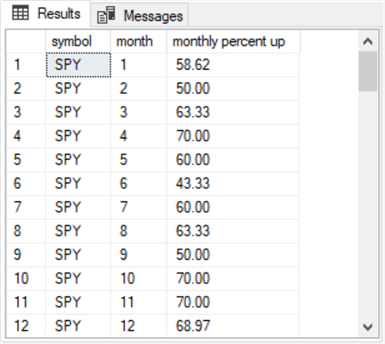
select * from #temp_seasonal_factors
The next two screenshots show the first and last twelve rows from the #temp_seasonal_factors table. The first twelve rows are for the SPY ticker symbol, and the last twelve rows are for the UDOW ticker symbol. The intermediate rows are for the remaining four ticker symbols.

- The next code excerpt for the seasonal_include_model focuses on
- An approach for adapting a stored procedure (compute_median_by_category) originally introduced and described in the “Two stored procedures for computing medians” section of a prior tip titled “T-SQL Starter Statistics Package for SQL Server“.
- The stored procedure was originally designed to compute medians for values within categories. For this tip,
- A category corresponds to a ticker symbol
- The values within a category correspond to the monthly percent up column values from the #temp_seasonal_factors table; this table is created and populated in the preceding script excerpt
- The stored procedure processes data from the ##table_for_median_by_category table; this table is created and populated by the preceding script
- After creating the stored procedure and populating ##table_for_median_by_category from the #temp_seasonal_factors table, the code excerpt invokes the compute_median_by_category stored procedure and saves its results set in the @tmpTable table variable
- Next, the code joins the ##table_for_median_by_category table to a derived table based on the @tmpTable table variable; the derived table name is my_table_variable. The results set from the join populates ##table_for_median_by_category_with_seasonal_include_indicator
- In the process of joining the two tables, the code adds a computed column named seasonal_include_idicator. The computed column has
- A value of 1 when the column_for_median column value from the ##table_for_median_by_category table is greater than median_by_category column value from the @tmpTable table variable
- A value of 0 otherwise
drop procedure if exists dbo.compute_median_by_category
go

create procedure compute_median_by_category
as
begin
   set nocount on;

   select
      *
   from
   (
      -- compute median by gc_dc_symbol
      -- distinct in select statement shows just one median per symbol
      select
         distinct category
        ,percentile_cont(.5)
            within group (order by column_for_median)
            over(partition by category) median_by_category
      from
      (
         select
            category
           ,column_for_median
         from ##table_for_median_by_category
      ) for_median_by_category
   ) for_median_by_category
   order by category

   return

end
go


-- create and populate ##table_for_median_by_category
-- from #temp_seasonal_factors
-- for processing by compute_median_by_category stored procedure
drop table if exists ##table_for_median_by_category
select symbol [category], [monthly percent up] [column_for_median]
into ##table_for_median_by_category
from #temp_seasonal_factors
order by #temp_seasonal_factors.month

-- optionally display  ##table_for_median_by_category
select * from ##table_for_median_by_category

-- invoke compute_median_by_category stored procedure
-- display category and median_by_category from @tmpTable
declare @tmpTable TABLE (category varchar(5), median_by_category real)

insert into @tmpTable
exec compute_median_by_category

select category, median_by_category from @tmpTable

drop table if exists ##table_for_median_by_category_with_seasonal_include_indicator

-- compute seasonal_include_indicator
select
 ##table_for_median_by_category.category
,column_for_median
,median_by_category
,case
   when column_for_median > my_table_variable.median_by_category then 1
   else 0
end seasonal_include_idicator

into ##table_for_median_by_category_with_seasonal_include_indicator
from ##table_for_median_by_category

join

(select category, median_by_category from @tmpTable) my_table_variable
on ##table_for_median_by_category.category = my_table_variable.category
Here are three results sets from the preceding script.
- The first pane shows the column values for the SPY ticker from the ##table_for_median_by_category table. There are five other sets of values in the full version of the results set for the first pane
- The second pane shows the six median values computed by the compute_median_by_category stored procedure and saved in the @tmpTable table variable
- The third pane shows the seasonal_include_indicator column values for the SPY ticker

Implementing the ensemble_model
The final component in an ensemble model is the one that brings all the other model components together into a single model. There are many potential approaches for implementing this final step.
- In this tip, there are just two AI model elements in the ensemble AI model.
- The first element is the close_gt_ema_10_model
- The second element is the seasonal_include_model
- This section describes an approach for combining the final results sets from each model element. The approach is to include results from the close_gt_ema_10_model that have start dates from months with seasonal_include_indicator column values of 1.
- Recall that seasonal_include_indicator column value of 1 reveals that the column_for_median column value is greater than the median_by_category column value
- By combining rows from the close_gt_ema_10_model results sets with start dates having a seasonal_include_indicator value of 1
The first pair of queries focus on seasonal factors. Two fresh tables are created and populated.
- The first query adds an identity column, my_id, to the ##table_for_median_by_category_with_seasonal_include_indicator table. The table with the freshly added column has a name of ##table_for_median_by_category_with_seasonal_include_indicator_with_my_id
- The second query adds another identity column to the #temp_seasonal_factors. The table with the freshly added column has a name of #temp_seasonal_factors_with_my_id
- Each of these tables has 72 rows — for 12 monthly dates for each of 6 tickers
-- my_id column values are for joining
-- ##table_for_median_by_category_with_seasonal_include_indicator_with_my_id with
-- #temp_seasonal_factors_with_my_id
-- to make month column values in same results set as one with seasonal_include_indicator values

drop table if exists ##table_for_median_by_category_with_seasonal_include_indicator_with_my_id

select identity(int,1,1) AS my_id, *
into ##table_for_median_by_category_with_seasonal_include_indicator_with_my_id
from
##table_for_median_by_category_with_seasonal_include_indicator_with_my_id
-- optionally display
select * from ##table_for_median_by_category_with_seasonal_include_indicator_with_my_id


drop table if exists #temp_seasonal_factors_with_my_id

select identity(int,1,1) AS my_id, *
into #temp_seasonal_factors_with_my_id
from #temp_seasonal_factors

-- optionally display #temp_seasonal_factors_with_my_id
select * from #temp_seasonal_factors_with_my_id
The next pair of select statements join the ##temp_with_close_and_close_lead_10_for_each_start_cycle_plus_duration_in_years table with the pair of results sets from the preceding script excerpt.
- The two select statements are identical, except for their where clauses
- The where clause in the first select statement extracts rows from the joined results set just for rows with a seasonal_include_idicator value of 1. For the data in this tip, there are 658 rows in this results set
- The where clause in the second select statement extracts rows from the joined results set just for rows with a seasonal_include_idicator value of 0. For the data in this tip, there are 639 rows in this results set
- The sum of 658 and 639 is a control total equal to the total number of buy/sell cycles in the close_gt_ema_10_model (1297)
- The select statements for these two results sets are nested in a subquery named for_month_and_seasonal_include_indicator_by_category
- Recall that ##temp_with_close_and_close_lead_10_for_each_start_cycle_plus_duration_in_years is a global temp table created in the code for the close_gt_ema_10_model. The use of a global temp table makes it possible for its contents to be accessed from any SQL file so long as the SQL file for creating the global temp table remains open
-- display ##temp_with_close_and_close_lead_10_for_each_start_cycle_plus_duration_in_years
-- for use with seasonal_include_model
-- from_close_gt_ema_10_model
-- joined to the seasonal_include_model
-- with seasonal_include_indicator = 1
select
.*
,for_month_and_seasonal_include_indicator_by_category.month
,for_month_and_seasonal_include_indicator_by_category.seasonal_include_idicator

from ##temp_with_close_and_close_lead_10_for_each_start_cycle_plus_duration_in_years

join

(
-- join tables with matching my_id columns to retrieve month column values
-- from #temp_seasonal_factors_with_my_id for use with
-- ##table_for_median_by_category_with_seasonal_include_indicator_with_my_id
select
#temp_seasonal_factors_with_my_id.month
,##table_for_median_by_category_with_seasonal_include_indicator_with_my_id.*
from #temp_seasonal_factors_with_my_id

join ##table_for_median_by_category_with_seasonal_include_indicator_with_my_id

on #temp_seasonal_factors_with_my_id.my_id =
   ##table_for_median_by_category_with_seasonal_include_indicator_with_my_id.my_id

) for_month_and_seasonal_include_indicator_by_category

on ##temp_with_close_and_close_lead_10_for_each_start_cycle_plus_duration_in_years.symbol =
   for_month_and_seasonal_include_indicator_by_category.category and
##temp_with_close_and_close_lead_10_for_each_start_cycle_plus_duration_in_years.month_number =
  for_month_and_seasonal_include_indicator_by_category.month
where seasonal_include_idicator = 1

------------------------------------------------------------------------------------------

-- display ##temp_with_close_and_close_lead_10_for_each_start_cycle_plus_duration_in_years
-- for use with seasonal_include_model
-- from_close_gt_ema_10_model
-- joined to the seasonal_include_model
-- with seasonal_include_indicator = 0
select
 ##temp_with_close_and_close_lead_10_for_each_start_cycle_plus_duration_in_years.*
,for_month_and_seasonal_include_indicator_by_category.month
,for_month_and_seasonal_include_indicator_by_category.seasonal_include_idicator

from ##temp_with_close_and_close_lead_10_for_each_start_cycle_plus_duration_in_years

join

(
-- join tables with matching my_id columns to retrieve month column values
-- from #temp_seasonal_factors_with_my_id for use with
-- ##table_for_median_by_category_with_seasonal_include_indicator_with_my_id
select
#temp_seasonal_factors_with_my_id.month
,##table_for_median_by_category_with_seasonal_include_indicator_with_my_id.*
from #temp_seasonal_factors_with_my_id

join ##table_for_median_by_category_with_seasonal_include_indicator_with_my_id

on #temp_seasonal_factors_with_my_id.my_id =
   ##table_for_median_by_category_with_seasonal_include_indicator_with_my_id.my_id

) for_month_and_seasonal_include_indicator_by_category

on ##temp_with_close_and_close_lead_10_for_each_start_cycle_plus_duration_in_years.symbol =
   for_month_and_seasonal_include_indicator_by_category.category and
##temp_with_close_and_close_lead_10_for_each_start_cycle_plus_duration_in_years.month_number =
  for_month_and_seasonal_include_indicator_by_category.month
where seasonal_include_idicator = 0
The next code excerpt creates and populates a temp table named ##temp_with_close_and_close_lead_10_for_each_start_cycle_plus_duration_in_years_with_seasonal_include_idicator_equals_1. This temp table serves as the source dataset for the report of performance from the ensemble_model.
- The select into statement immediately after the drop table if exists statement creates and populates the ##temp_with_close_and_close_lead_10_for_each_start_cycle_plus_duration_in_years_with_seasonal_include_idicator_equals_1 table
- Five of the six select list items are from the ##temp_with_close_and_close_lead_10_for_each_start_cycle_plus_duration_in_years source table
- The sixth and final select list item is from the for_month_and_seasonal_include_indicator_by_category subquery
- The month_and_seasonal_include_indicator_by_category subquery contains selected columns from a join of the #temp_seasonal_factors_with_my_id table and the ##table_for_median_by_category_with_seasonal_include_indicator_with_my_id table
- The where clause in the select into statement has a criterion of seasonal_include_idicator = 1
- The optional select statement at the end of the excerpt below can display the contents of ##temp_with_close_and_close_lead_10_for_each_start_cycle_plus_duration_in_years_with_seasonal_include_idicator_equals_1
drop table if exists
 ##temp_with_close_and_close_lead_10_for_each_start_cycle_plus_duration_in_years_with_seasonal_include_idicator_equals_1


-- create, populate, and optionally display
-- ##temp_with_close_and_close_lead_10_for_each_included_start_cycle_plus_duration_in_years
-- for use with seasonal_include_model
-- from_close_gt_ema_10_model
-- joined to the seasonal_include_model
-- with seasonal_include_indicator = 1
select
 ##temp_with_close_and_close_lead_10_for_each_start_cycle_plus_duration_in_years.symbol
,##temp_with_close_and_close_lead_10_for_each_start_cycle_plus_duration_in_years.date
,##temp_with_close_and_close_lead_10_for_each_start_cycle_plus_duration_in_years.[close]
,##temp_with_close_and_close_lead_10_for_each_start_cycle_plus_duration_in_years.close_lead_10
,##temp_with_close_and_close_lead_10_for_each_start_cycle_plus_duration_in_years.duration_in_years
,for_month_and_seasonal_include_indicator_by_category.seasonal_include_idicator

into ##temp_with_close_and_close_lead_10_for_each_start_cycle_plus_duration_in_years_with_seasonal_include_idicator_equals_1

from ##temp_with_close_and_close_lead_10_for_each_start_cycle_plus_duration_in_years

join

(
-- join tables with matching my_id columns to retrieve month column values
-- from #temp_seasonal_factors_with_my_id for use with
-- ##table_for_median_by_category_with_seasonal_include_indicator_with_my_id
select
#temp_seasonal_factors_with_my_id.month
,##table_for_median_by_category_with_seasonal_include_indicator_with_my_id.*
from #temp_seasonal_factors_with_my_id

join ##table_for_median_by_category_with_seasonal_include_indicator_with_my_id

on #temp_seasonal_factors_with_my_id.my_id =
   ##table_for_median_by_category_with_seasonal_include_indicator_with_my_id.my_id

) for_month_and_seasonal_include_indicator_by_category

on ##temp_with_close_and_close_lead_10_for_each_start_cycle_plus_duration_in_years.symbol =
   for_month_and_seasonal_include_indicator_by_category.category and
##temp_with_close_and_close_lead_10_for_each_start_cycle_plus_duration_in_years.month_number =
  for_month_and_seasonal_include_indicator_by_category.month
where seasonal_include_idicator = 1


-- optionally display next-to-final results set for seasonal_include model
select *
 from ##temp_with_close_and_close_lead_10_for_each_start_cycle_plus_duration_in_years_with_seasonal_include_idicator_equals_1
The final script for the ensemble model appears below. The script excerpt for the ensemble_model computes summary values for each of the six ticker symbols tracked in this tip. There are six columns in the summary results table (#temp_summary).
The layout and design of the summary values for the six tickers from the ensemble_model are the same as from the summary table for the close_gt_ema_10_model. However, the actual source data for the summary values report is different for the ensemble_model versus the close_gt_ema_10_model. This is because of design feature differences between the two models.
- Both models start with the same set of buy/sell cycles. This is because both models have the same set of initial rules for identifying buy/sell cycles.
- However, for the data tracked in this tip, the ensemble_model discards about half of the initial buy/sell cycles. This is because the ensemble_model filters out about half the initial buy/sell cycles by retaining just those that have start dates in months with a monthly percent up in close price that is greater than the median monthly percent up for a symbol (also called a category)
- The close_gt_ema_10_model retains all buy/sell cycles whether or not they start in months with an above median monthly percent up in their close values
- Aside from this seasonality issue, the ensemble_model is identical to the close_gt_ema_10_model
- In terms of the actual code within the script excerpts
- The ensemble_model summary report pulls its underlying values from ##temp_with_close_and_close_lead_10_for_each_start_cycle_plus_duration_in_years_with_seasonal_include_idicator_equals_1, which, in turn, derives its values from the ##temp_with_close_and_close_lead_10_for_each_start_cycle_plus_duration_in_years table
- The close_gt_ema_10_model pulls its underlying values from #temp_with_close_and_close_lead_10_for_each_start_cycle_plus_duration_in_years
-- create and populate #temp_summary for ensemble_model
-- with seasonal_include_idicator = 1

drop table if exists #temp_summary

-- setup for populating #temp_summary
-- with data for DIA symbol
declare @symbol nvarchar(10) = 'DIA'
declare @first_date date =
   (select min(date)
    from ##temp_with_close_and_close_lead_10_for_each_start_cycle_plus_duration_in_years_with_seasonal_include_idicator_equals_1
   where symbol = @SYMBOL)
declare @last_date date =
   (select max(date)
   from ##temp_with_close_and_close_lead_10_for_each_start_cycle_plus_duration_in_years_with_seasonal_include_idicator_equals_1
   where symbol = @SYMBOL)
declare @first_close dec (19,4) =
   (select [close]
   from ##temp_with_close_and_close_lead_10_for_each_start_cycle_plus_duration_in_years_with_seasonal_include_idicator_equals_1
   where symbol = @SYMBOL and
   date = @first_date)
declare @last_close_lead_10 dec (19,4) =
   (select close_lead_10
   from ##temp_with_close_and_close_lead_10_for_each_start_cycle_plus_duration_in_years_with_seasonal_include_idicator_equals_1
   where symbol = @SYMBOL and
   date = @last_date)
declare @last_duration_in_years dec(19,4) =
   (
   select duration_in_years
   from ##temp_with_close_and_close_lead_10_for_each_start_cycle_plus_duration_in_years_with_seasonal_include_idicator_equals_1
   where symbol = @SYMBOL and
   date = @last_date
   )

-- populate #temp_summary for DIA
select @symbol [@symbol], @first_close [@first_close], @last_close_lead_10 [@last_close_lead_10]
   ,@last_duration_in_years [@last_duration_in_years]
   , @last_close_lead_10 - @first_close [change]
   ,cast((power(( @last_close_lead_10/@first_close),(1.0/@last_duration_in_years))-1)*100 as dec(19,2)) cagr
into #temp_summary


-- setup to populate #temp_summary for QQQ
 set @symbol = 'QQQ'
 set @first_date =
   (select min(date)
    from ##temp_with_close_and_close_lead_10_for_each_start_cycle_plus_duration_in_years
   where symbol = @SYMBOL)
 set @last_date =
   (select max(date)
   from ##temp_with_close_and_close_lead_10_for_each_start_cycle_plus_duration_in_years
   where symbol = @SYMBOL)
set @first_close =
   (select [close]
   from ##temp_with_close_and_close_lead_10_for_each_start_cycle_plus_duration_in_years
   where symbol = @SYMBOL and
   date = @first_date)
set @last_close_lead_10 =
   (select close_lead_10
   from ##temp_with_close_and_close_lead_10_for_each_start_cycle_plus_duration_in_years
   where symbol = @SYMBOL and
   date = @last_date)
set @last_duration_in_years =
   (
   select duration_in_years
   from ##temp_with_close_and_close_lead_10_for_each_start_cycle_plus_duration_in_years
   where symbol = @SYMBOL and
   date = @last_date
   )

-- populate #temp_summary for QQQ
insert into #temp_summary
select @symbol [@symbol], @first_close [@first_close], @last_close_lead_10 [@last_close_lead_10]
   ,@last_duration_in_years [@last_duration_in_years]
   , @last_close_lead_10 - @first_close [change]
   ,cast((power(( @last_close_lead_10/@first_close),(1.0/@last_duration_in_years))-1)*100 as dec(19,2)) cagr


-- setup to populate #temp_summary for SPXL
 set @symbol = 'SPXL'
 set @first_date =
   (select min(date)
    from ##temp_with_close_and_close_lead_10_for_each_start_cycle_plus_duration_in_years
   where symbol = @SYMBOL)
 set @last_date =
   (select max(date)
   from ##temp_with_close_and_close_lead_10_for_each_start_cycle_plus_duration_in_years
   where symbol = @SYMBOL)
set @first_close =
   (select [close]
   from ##temp_with_close_and_close_lead_10_for_each_start_cycle_plus_duration_in_years
   where symbol = @SYMBOL and
   date = @first_date)
set @last_close_lead_10 =
   (select close_lead_10
   from ##temp_with_close_and_close_lead_10_for_each_start_cycle_plus_duration_in_years
   where symbol = @SYMBOL and
   date = @last_date)
set @last_duration_in_years =
   (
   select duration_in_years
   from ##temp_with_close_and_close_lead_10_for_each_start_cycle_plus_duration_in_years
   where symbol = @SYMBOL and
   date = @last_date
   )

-- populate #temp_summary for SPXL
insert into #temp_summary
select @symbol [@symbol], @first_close [@first_close], @last_close_lead_10 [@last_close_lead_10]
   ,@last_duration_in_years [@last_duration_in_years]
   , @last_close_lead_10 - @first_close [change]
   ,cast((power(( @last_close_lead_10/@first_close),(1.0/@last_duration_in_years))-1)*100 as dec(19,2)) cagr


-- setup to populate #temp_summary for SPY
 set @symbol = 'SPY'
 set @first_date =
   (select min(date)
    from ##temp_with_close_and_close_lead_10_for_each_start_cycle_plus_duration_in_years
   where symbol = @SYMBOL)
 set @last_date =
   (select max(date)
   from ##temp_with_close_and_close_lead_10_for_each_start_cycle_plus_duration_in_years
   where symbol = @SYMBOL)
set @first_close =
   (select [close]
   from ##temp_with_close_and_close_lead_10_for_each_start_cycle_plus_duration_in_years
   where symbol = @SYMBOL and
   date = @first_date)
set @last_close_lead_10 =
   (select close_lead_10
   from ##temp_with_close_and_close_lead_10_for_each_start_cycle_plus_duration_in_years
   where symbol = @SYMBOL and
   date = @last_date)
set @last_duration_in_years =
   (
   select duration_in_years
   from ##temp_with_close_and_close_lead_10_for_each_start_cycle_plus_duration_in_years
   where symbol = @SYMBOL and
   date = @last_date
   )

-- populate #temp_summary for SPY
insert into #temp_summary
select @symbol [@symbol], @first_close [@first_close], @last_close_lead_10 [@last_close_lead_10]
   ,@last_duration_in_years [@last_duration_in_years]
   , @last_close_lead_10 - @first_close [change]
   ,cast((power(( @last_close_lead_10/@first_close),(1.0/@last_duration_in_years))-1)*100 as dec(19,2)) cagr


-- setup to populate #temp_summary for TQQQ
 set @symbol = 'TQQQ'
 set @first_date =
   (select min(date)
    from ##temp_with_close_and_close_lead_10_for_each_start_cycle_plus_duration_in_years
   where symbol = @SYMBOL)
 set @last_date =
   (select max(date)
   from ##temp_with_close_and_close_lead_10_for_each_start_cycle_plus_duration_in_years
   where symbol = @SYMBOL)
set @first_close =
   (select [close]
   from ##temp_with_close_and_close_lead_10_for_each_start_cycle_plus_duration_in_years
   where symbol = @SYMBOL and
   date = @first_date)
set @last_close_lead_10 =
   (select close_lead_10
   from ##temp_with_close_and_close_lead_10_for_each_start_cycle_plus_duration_in_years
   where symbol = @SYMBOL and
   date = @last_date)
set @last_duration_in_years =
   (
   select duration_in_years
   from ##temp_with_close_and_close_lead_10_for_each_start_cycle_plus_duration_in_years
   where symbol = @SYMBOL and
   date = @last_date
   )

-- populate #temp_summary for UDOW
insert into #temp_summary
select @symbol [@symbol], @first_close [@first_close], @last_close_lead_10 [@last_close_lead_10]
   ,@last_duration_in_years [@last_duration_in_years]
   , @last_close_lead_10 - @first_close [change]
   ,cast((power(( @last_close_lead_10/@first_close),(1.0/@last_duration_in_years))-1)*100 as dec(19,2)) cagr

-- setup to populate #temp_summary for UDOW
 set @symbol = 'UDOW'
 set @first_date =
   (select min(date)
    from ##temp_with_close_and_close_lead_10_for_each_start_cycle_plus_duration_in_years
   where symbol = @SYMBOL)
 set @last_date =
   (select max(date)
   from ##temp_with_close_and_close_lead_10_for_each_start_cycle_plus_duration_in_years
   where symbol = @SYMBOL)
set @first_close =
   (select [close]
   from ##temp_with_close_and_close_lead_10_for_each_start_cycle_plus_duration_in_years
   where symbol = @SYMBOL and
   date = @first_date)
set @last_close_lead_10 =
   (select close_lead_10
   from ##temp_with_close_and_close_lead_10_for_each_start_cycle_plus_duration_in_years
   where symbol = @SYMBOL and
   date = @last_date)
set @last_duration_in_years =
   (
   select duration_in_years
   from ##temp_with_close_and_close_lead_10_for_each_start_cycle_plus_duration_in_years
   where symbol = @SYMBOL and
   date = @last_date
   )

-- populate #temp_summary for UDOW
insert into #temp_summary
select @symbol [@symbol], @first_close [@first_close], @last_close_lead_10 [@last_close_lead_10]
   ,@last_duration_in_years [@last_duration_in_years]
   , @last_close_lead_10 - @first_close [change]
   ,cast((power(( @last_close_lead_10/@first_close),(1.0/@last_duration_in_years))-1)*100 as dec(19,2)) cagr

-- display #temp_summary across all symbols
   select * from #temp_summary
Here is the results set from the preceding script. There are two main summary metrics. The cagr returns the average annual growth rate for which an investment strategy is evaluated. The change value reflects the difference between @last_close_lead_10 and @first_close.
- By the cagr metric
- The TQQQ ticker gave the best return on invested capital
- The DIA ticker gave the worst return on invested capital
- The three tickers for leveraged ETFs gave returns that were more than three times as large as those for unleveraged ETFs. As you can see, the @last_duration_in_years column values are much larger for the unleveraged securities (DIA, QQQ, SPY) than for the leveraged securities (SPXL, TQQQ, UDOW)
- By the change metric
- Returns were five times (or larger) for the unleveraged securities (DIA, QQQ, SPY) than for the leveraged securities (SPXL, TQQQ, UDOW)
- As with the cagr metric, this outcome is driven by the fact that the duration in years was much greater for the unleveraged securities than for the leveraged securities
- The change metric column below has identical values for all ticker symbols except for the DIA ticker
- The change metric for the DIA ticker from the ensemble_model has a value of 237.3262
- The change metric for the DIA ticker from the close_gt_ema_10_model has a value of 248.0137; the summary report for the close_gt_ema_10_model appears at the end of the “Implementing the close_gt_ema_10_model” section
- The reason the DIA change metric value is less for the ensemble_model summary report than for the close_gt_ema_10_model summary report is because the @first_close value is larger for the ensemble model than for the close_gt_ema_10_model; the seasonality rules for the ensemble_model causes it to choose a larger @first_close value than does the close_gt_ema_10_model. The larger @first_close value reduces the @last_close_lead_10 value by a greater amount for the ensemble_model than for the close_gt_ema_10_model

There is at least one important difference between the close_gt_ema_10 model versus the ensemble_model that is not indicated by a comparison of summary tables from the two models.
- There are about 660 buy/sell cycles selected by the ensemble_model
- In contrast, there are about 1300 buy/sell cycles selected by the close_gt_ema_10_model
- This means that the same amount of invested dollars for the ensemble_model may be able to return about twice the gain as from the close_gt_ema_10_model because it has about twice as many tries to achieve an enhanced return
Next Steps
The next step after reading this tip is to decide if you want a hands-on experience with the techniques demonstrated in this tip. You can get the code you need for hands-on experience from the code windows in the tip. However, if you want to run the code exactly as it is described in the tip, then you also need the symbol_date and yahoo_finance_ohlcv_values_with_symbol tables.
The source data and the T-SQL script for importing the source data to the symbol_date table is available from the download for a prior tip titled “SQL Server Data Mining for Leveraged Versus Unleveraged ETFs as a Long-Term Investment“. This prior tip also includes the source code for the symbol_date table’s primary key constraint.
Another approach is to adapt the code excerpts provided in this tip to data derived from your business. All you need for this approach is a dataset that documents some decisions and some source data columns that are likely to serve as inputs for AI models about the decisions. In this tip, the decision is about when to buy and sell securities. However, the decision can be about any type of decision, such as when to buy new materials and how much of them to buy for replenishing inventory items for a manufacturing or sales business. This approach removes the need to copy CSV files from a prior tip and then load the contents of the CSV files into a SQL Server table. With this approach, all you need to do is copy one or more database objects from your production database to your newly created ensemble AI model.

Rick Dobson is a SQL Server professional with decades of T-SQL experience that includes authoring books, running a national seminar practice, working for businesses on finance and healthcare development projects, and serving as a regular contributor to MSSQLTips.com. He has been a practicing Python developer for more than the past half decade – with a special emphasis for data visualization and ETL tasks with JSON and CSV files. His most recent professional passions include financial time series data and analyses, AI models, and statistics. If you are interested in growing your skills in any of these areas especially as they relate to financial securities, consider visiting his blog at https://securitytradinganalytics.blogspot.com/2023/12/.
- MSSQLTips Awards: Leadership (200+ tips) – 2025 | Author of the Year Contender – 2017-2024