Problem
I would like to know how to program artificial intelligence (AI) for time series data in SQL Server. Please describe an AI model for making decisions about time series data. Next, present T-SQL code on how to program the AI model. Conclude with a summary of selected results evaluating the success of AI model decisions.
Solution
Data science is a hot topic among computer professionals. One area within data science involves specifying an AI model to make decisions based on data. This tip demonstrates it can be relatively uncomplicated to specify an AI model. In this tip, you’ll see some answers to question like these:
- How to specify a model for making decisions about time series data
- How to program the model with T-SQL for data stored in a SQL Server instance
- How to review results from the model to evaluate the success of the model-based decisions
MSSQLTips.com offers several prior tips on how to collect time series data and organize them for use within SQL Server (here, here, and here). Building an AI model is a use case for time series data.
An AI model specification for financial time series data
AI is for making decisions about data. AI can make projections like: will it rain tomorrow? or when will coronavirus fatalities peak? This tip demonstrates how to specify, build, and evaluate an AI model to find a buy price that is less than one or more sell prices for a stock symbol. When the buy price is less than one of the sell prices, then the AI model decided to buy a security and sell it subsequently for a profit.
The following script shows some code to compute change values for close prices in typical open-high-low-close-volume time series data.
- The time series data reside in the yahoo_prices_valid_vols_only table from the for_csv_from_python database.
- Each row is for a specific symbol and trading date; the script selects the NBIX symbol in a where clause.
- Each date value for a symbol has a collection of open, high, low, close, and volume values.
- A top 10 clause restricts the results to the first ten rows by date.
- The select statement in the bottom portion of the script computes change and change_percent values relative to the first close price.
- A declare statement towards the top of the script returns the first close price as a local variable named @1stclose.
- Change and change_percent values are based on simple expressions. These kinds of expressions are especially handy for evaluating the performance of some AI models.
-- An example computing change and change percent
-- for time series values
use for_csv_from_python
go

declare @1stclose money =
(
select [close]
from [yahoo_prices_valid_vols_only]
where [symbol] = 'NBIX' and date = '2009-01-02'
);

-- list first 10 time series data
-- plus, a pair of columns of computed change values
select top 10
       [Date]
      ,[Symbol]
      ,[Open]
      ,[High]
      ,[Low]
      ,[Close]
      ,[Volume]
      ,([Close] - @1stclose) change
      ,((([Close] - @1stclose)/[Close])*100) change_percent
from
[dbo].[yahoo_prices_valid_vols_only]
where symbol = 'NBIX'
Here’s the output from the preceding script.
- The change column value is the close price for a row less the value of @1stclose.
- If the close value for a row is greater than the value for @1stclose, then that row has a greater value than the close price for the first row.

The task for this tip’s AI model is to find a set of contiguous rows where many or all the rows after the first row have a price value that is greater than the value for the close price for the initial row. There are multiple prices for each row, such as close price and open price.
- This tip’s AI model uses the close price along with exponential moving averages to find sets of contiguous rows with rising prices on average.
- The model uses the open price to specify buy and sell prices for the first and last prices within each set of rows.
The AI model’s goal is to start at a relatively lower-priced row and end at a relatively higher-priced row. The model uses relationships between exponential moving averages for the close price for each row. An exponential moving average is a specialized weighted moving average for a set of rows. A ten-period exponential moving average is the exponentially weighted moving average of the most recent ten close values, ending with the close price for the current row. Similarly, a thirty-period moving average is the exponentially weighted moving average of the most recent thirty close values. If the ten-period moving average is greater than the thirty-period moving average, then the most recent ten close values are greater on average than the most recent thirty close values. This preceding tip Exponential Moving Average Calculation in SQL Server drills down on how to compute exponential moving averages with different period lengths. Especially examine the tip for a pair of stored procedures that computes exponential moving averages; the stored procedure names are usp_ema_computer and insert_computed_emas. Here’s a web page with an overview of how to use different types of averages, including exponential moving averages, with financial time series data.
This tip’s AI model uses four different exponential moving averages to identify a set of contiguous rows with rising values on average. The relationships among the moving averages is as follows.
- The ten-period exponential moving average must be greater than the thirty-period moving average.
- The thirty-period exponential moving average must be greater than the fifty-period moving average.
- The fifty-period exponential moving average must be greater than the two-hundred-period moving average.
This prior tip Analyze Relationship Between Two Time Series in SQL Server drills down on how to use T-SQL to confirm an uptrend among the four exponential moving averages.
When two or more contiguous rows meet these requirements, then the time series values are increasing across the set of rows. The more contiguous rows with all three relationships, the more the general tendency for prices to rise from the least recent row through the most recent row.
This tip’s AI model includes another pair of requirements.
- The open price for the least recent row is the buy_price.
- The open price for the most recent row (or any row following the buy price row) can serve as the sell_price.
Some T-SQL code for an AI model
The time series data for this tip was initially organized and saved in a prior tip. Recall that the source data resides in the yahoo_prices_valid_vols_only table of the dbo schema within the for_csv_from_python database. This data source is referenced in the script from the previous section. There are several additional regular tables, temp tables, and a table variable that holds supplementary data required for the execution of the AI model.
Here’s the code for creating the two regular tables.
- The date_symbol_close_period_length_ema table in the dbo schema derives values for its date, symbol, and close columns from the yahoo_prices_valid_vols_only table. The “period length”, and exponential moving average (ema) columns are derived from a table of ema values. Any time series value can have one or more exponential moving averages each with a different period length. The period length designates the number of prior periods in addition to the current period used to compute a moving average. After the create table statement for the date_symbol_close_period_length_ema table, the code creates a fresh version of the primary key for the table.
- The primary key for the date_symbol_close_period_length_ema table is based on an index derived from symbol, date, and period length column values in the table.
- Rows in the table are unique by the combination of these three column values.
- Another regular SQL Server table populated by the AI model has the name stored_trades in the dbo schema. The stored_trades table contains data from three sources.
- The first set of columns (from symbol through volume) are populated with values from the original time series source data.
- A second set of columns are populated from re-shaped data from the date_symbol_close_period_length_ema table.
- The source data are normalized by symbol, date, and period length. The source data contains a single ema column.
- The re-shaped data are pivoted. The pivoted data displays exponential values in multiple columns – one column per period length.
- The AI model marks rows from the original time values to identify rows with rising exponential moving averages from the two-hundred period length exponential moving average through to the ten-period length exponential moving average.
- If a row does not have rising exponential moving averages, then identifier columns (all_uptrending_emas and trending_status) are set to indicate the moving averages are not rising from the longest period length to the shortest period length. Similarly, rows with rising exponential moving averages receive different values in their identifier columns.
- Contiguous rows with rising exponential moving averages are segmented into sets so that each set starts with an initial date for a symbol that begins a set of contiguous rows with rising exponential moving averages. Similarly, the end of contiguous rows with rising exponential moving averages is also identified.
- The buy_price and sell_price column values are populated, respectively, with the open price values from the original time series source data for the least recent and most recent row in each set. Other rows for these two columns in the table are left with null values.
-- specify the default database reference
use for_csv_from_python
go

-- Create two regular tables for AI model
-- create and populate close_emas_trending_status_by_date_symbol

-- create a fresh copy of a table to store
-- underlying time series values (close prices)
-- and their exponential moving averages with different period lengths
begin try
   drop table [dbo].[date_symbol_close_period_length_ema]
end try
begin catch
   print '[dbo].[date_symbol_close_period_length_ema] is not available to drop'
end catch

create table [dbo].[date_symbol_close_period_length_ema](
   [date] [date] NOT NULL,
   [symbol] [nvarchar](10) NOT NULL,
   [close] [money] NULL,
   [period length] [float] NOT NULL,
   [ema] [money] NULL
)

-- add primary key constraint named symbol_date_period_length
-- to date_symbol_close_period_length_ema
begin try
alter table [dbo].[date_symbol_close_period_length_ema]
  drop constraint [symbol_date_period_length]
end try
begin catch
  print 'primary key not available to drop'
end catch

-- add a constraint to facilitate retrieving saved emas
alter table [dbo].[date_symbol_close_period_length_ema]
  add constraint symbol_date_period_length
    primary key(symbol, date, [period length]);


-- create a fresh copy of a table to store
-- trades for a symbol with buy and sell
-- prices and dates
begin try
   drop table [dbo].stored_trades
end try
begin catch
   print '[dbo].stored_trades is not available to drop'
end catch

create table [dbo].stored_trades(
   [symbol] [nvarchar](10) NOT NULL,
   [date] [date] NOT NULL,
   [open] [money] NULL,
   [high] [money] NULL,
   [low] [money] NULL,
   [close] [money] NULL,
   [volume] [bigint] NULL,
   [ema_10] [money] NULL,
   [ema_30] [money] NULL,
   [ema_50] [money] NULL,
   [ema_200] [money] NULL,
   [all_uptrending_emas] [int] NULL,
   [trending_status] [varchar](18) NULL,
   [buy_price] [money] NULL,
   [sell_price] [money] NULL)
go
The next block of code for implementing the AI model populates a data source (@symbol_table) with a set of four symbols (NBIX, BKNG, NFLX, and ULTA). These four symbols are used to help populate the stored_trades table; this table can be used for analyzing the performance of the model. A table variable is used for storing the symbols. The population of the table variable is followed by a while loop that successively invokes the compute_and_save_buys_and_sells_for_symbol stored proc from the dbo schema for each of the four symbols. This stored procedure implements the AI model.
-- declare @symbol table
declare @symbol_table table(
     symbol_id int
    ,symbol nvarchar(10) NOT NULL
);

insert into @symbol_table
select *
from
(
select 1 symbol_id_nbr, 'NBIX' symbol
union
select 2 symbol_id_nbr, 'BKNG' symbol
union
select 3 symbol_id_nbr, 'NFLX' symbol
union
select 4 symbol_id_nbr, 'ULTA' symbol
) symbols_for_@symbol_table

-- loop code
declare @initial_loop_id int = 1, @last_loop_id int = 4, @loop_index int = 1, @symbol nvarchar(10)

while @loop_index <= @last_loop_id
begin

   select @symbol=symbol from @symbol_table where symbol_id = @loop_index
   exec [dbo].[compute_and_save_buys_and_sells_for_symbol]@symbol
   set @loop_index = @loop_index + 1

end
As just mentioned, the main implementation code for the AI model occurs in the compute_and_save_buys_and_sells_for_symbol stored procedure; the stored procedure’s create procedure statement appears next.
- The procedure starts by accepting one input parameter named @symbol. This stored procedure operates with whatever value is passed to its input parameter. For this demonstration of the model, the input parameter values are successively NBIX, BKNG, NFLX, and ULTA. With each successive run of the model, a set of rows are added to the stored_trades table for the current input parameter value.
- The stored procedure performs five successive steps. Highlights for each step are mentioned in the next set of bullets.
- Step 1 invokes the insert_computed_emas stored procedure within the dbo schema. This stored procedure populates the date_symbol_close_period_length_ema table for the input parameter value in @symbol. The insert_computed_emas stored procedure invoked in step 1 is briefly described in the “An AI model specification for financial time series data” section of this tip that also references a prior tip with in-depth coverage of the procedure’s code and operation.
- Step 2 re-shapes the ema values from the date_symbol_close_period_length_ema table and adds a new column. The output from step 2 is saved in the #for_@symbol_tests temp table. The date_symbol_close_period_length_ema table stores ema values in a normalized way for symbol, date, and period length values. Recall that the lengths are for ten periods, thirty periods, fifty periods, and two hundred periods. The #for_@symbol_tests table stores symbol, date, and close values along with separate columns for each ema values based on one of the four period lengths. After re-arranging the ema values, a case statement calculates all_uptrending_emas column values.
- This computed value is 1 when the ema column values for a row increase consistently from the two-hundred-period-length ema column through to the ten-period-length ema column.
- Otherwise, the computed value is 0.
- Step 3 uses the #for_@symbol_tests table as its source data. The main function of step 3 is to calculate via a case statement a new column based on its source data – with a special focus on all_uptrending_emas column values for current, prior, and next period rows. The lead function retrieves the next row’s column value relative to the current row, and the lag function retrieves the prior row’s column value relative to the current row. The new column has the name trending_status. The key trending_status values identify the beginning, middle, or end of either an uptrend or downtrend of ema values. The step 3 results set with the values from its source data along with the freshly computed trending_status column values are stored in the #close_emas_trending_status_by_date_symbol temp table.
- Next, step 4 left joins the ema column values and trending_status column values from the #close_emas_trending_status_by_date_symbol temp table to the original time series source data in the yahoo_prices_valid_vols_only table. The joined results set from step 4 is stored in the #yahoo_prices_valid_vols_only_joined_with_emas_and_trending_status temp table.
- Finally, step 5 accepts the data from the #yahoo_prices_valid_vols_only_joined_with_emas_and_trending_status temp table and adds two new columns. There are no additional steps to the AI model after step 5. Its output for the current input parameter value is added via an insert into statement to the stored_trades table. The new column names and values are as follows.
- The buy_price column value is the open price on the first date after the start of an uptrend. Otherwise, the buy_price column value is implicitly null (unspecified).
- The sell_price column value is the open price on the first date after the beginning of a downtrend. Otherwise, the sell_price is implicitly null.
-- create stored proc to compute buy and sell prices and dates based on emas
create procedure [dbo].[compute_and_save_buys_and_sells_for_symbol]
   -- Add the parameters for the stored procedure here
    @symbol nvarchar(10)  -- for example, assign as 'GOLD'

as

begin

-----------------------------------------------------------------------------------------
   -- step 1
   -- run stored procs to save computed emas for a symbol
   -- this step add rows to the [dbo].[date_symbol_close_period_length_ema]
   -- table with emas for the time series values with a symbol value of @symbol
   exec dbo.insert_computed_emas@symbol

--------------------------------------------------------------------------------------------
   -- step 2
   -- extract and join one column at a time
   -- for selected emas (ema_10, ema_30, ema_50, ema_200)
   -- for @symbol local variable

   -- also add all_uptrending_emas computed field
   -- to #for_@symbol_tests temp table
   -- value of 1 for all uptrending emas on a date
   -- value of 0 otherwise

   begin try
      drop table #for_@symbol_tests
   end try
   begin catch
      print '#for_@symbol_tests not available'
   end catch


   select
    symbol_10.*
   ,symbol_30.ema_30
   ,symbol_50.ema_50
   ,symbol_200.ema_200
   ,
    case
    when
      symbol_10.ema_10 > symbol_30.ema_30
      and ema_30 > ema_50
      and ema_50 > ema_200
      then 1
    else 0
    end all_uptrending_emas

   into #for_@symbol_tests
   from
   (
   -- extract emas with 10. 30, 50, and 200 period lengths
   select date, symbol, [close], ema ema_10
   from [dbo].[date_symbol_close_period_length_ema]
   where symbol = @symbol and [period length] = 10) symbol_10

   inner join

   (select date, symbol, [close], ema ema_30
   from [dbo].[date_symbol_close_period_length_ema]
   where symbol = @symbol and [period length] = 30) symbol_30

   on symbol_10.DATE = symbol_30.DATE

   inner join

   (select date, symbol, [close], ema ema_50
   from [dbo].[date_symbol_close_period_length_ema]
   where symbol = @symbol and [period length] = 50) symbol_50

   on symbol_10.DATE = symbol_50.DATE

   inner join

   (select date, symbol, [close], ema ema_200
   from [dbo].[date_symbol_close_period_length_ema]
   where symbol = @symbol and [period length] = 200) symbol_200

   on symbol_10.DATE = symbol_200.DATE

   --select * from #for_@symbol_tests order by date

--------------------------------------------------------------------------------------------
   -- step 3
   -- add computed trending_status field to
   -- #close_emas_trending_status_by_date_symbol temp table
   -- which is based on #for_@symbol_tests temp table

   begin try
      drop table #close_emas_trending_status_by_date_symbol
   end try
   begin catch
      print '#close_emas_trending_status_by_date_symbol not available to drop'
   end catch

   declare @start_date date = '2009-01-02', @second_date date = '2009-01-05'

   -- mark and save close prices and emas with ema trending_status
   select
    symbol
   ,date
   --,[close]
   ,ema_10
   ,ema_30
   ,ema_50
   ,ema_200
   ,all_uptrending_emas
   ,case
     when date in(@start_date, @second_date) then NULL

     when all_uptrending_emas = 1 and
            lag(all_uptrending_emas,1) over(order by date) = 0
            then 'start uptrend'
     when all_uptrending_emas = 1 and
            lead(all_uptrending_emas,1) over(order by date) = 1
            then 'in uptrend'
     when all_uptrending_emas = 1 and
            lead(all_uptrending_emas,1) over(order by date) = 0
            then 'end uptrend'
     when all_uptrending_emas = 0 and
            lag(all_uptrending_emas,1) over(order by date) = 1
            then 'start not uptrend'
     when all_uptrending_emas = 0 and
            lead(all_uptrending_emas,1) over(order by date) = 0
            then 'in not uptrend'
     when all_uptrending_emas = 0 and
            lead(all_uptrending_emas,1) over(order by date) = 1
            then 'end not uptrend'

     when isnull(lead(all_uptrending_emas,1) over(order by date),1) = 1
            then 'end of time series'
   end trending_status

   into #close_emas_trending_status_by_date_symbol
   from #for_@symbol_tests
   order by date

   --select * from #close_emas_trending_status_by_date_symbol order by date
--------------------------------------------------------------------------------------------
   -- step 4
   -- populate #yahoo_prices_valid_vols_only_joined_with_emas_and_trending_status with
   -- the basic time series data

   -- with each symbol having a succession of trading date rows
   -- with open, high, low, close price values and
   -- shares exchanged (volume) for each trading date

   -- with left join to close_emas_trending_status_by_date_symbol for emas
   -- and all_uptrending_emas plus trending status values

   begin try
      drop table
      #yahoo_prices_valid_vols_only_joined_with_emas_and_trending_status
   end try
   begin catch
      print '#yahoo_prices_valid_vols_only_joined_with_emas_and_trending_status
            not available to drop'
   end catch

   select
    [dbo].yahoo_prices_valid_vols_only.symbol
   ,[dbo].yahoo_prices_valid_vols_only.date
   ,[dbo].yahoo_prices_valid_vols_only.[open]
   ,[dbo].yahoo_prices_valid_vols_only.high
   ,[dbo].yahoo_prices_valid_vols_only.low
   ,[dbo].yahoo_prices_valid_vols_only.[close]
   ,[dbo].yahoo_prices_valid_vols_only.volume
   ,#close_emas_trending_status_by_date_symbol.ema_10
   ,#close_emas_trending_status_by_date_symbol.ema_30
   ,#close_emas_trending_status_by_date_symbol.ema_50
   ,#close_emas_trending_status_by_date_symbol.ema_200
   ,#close_emas_trending_status_by_date_symbol.all_uptrending_emas
   ,#close_emas_trending_status_by_date_symbol.trending_status

   into #yahoo_prices_valid_vols_only_joined_with_emas_and_trending_status
   from   [dbo].[yahoo_prices_valid_vols_only]
   left join #close_emas_trending_status_by_date_symbol
   on yahoo_prices_valid_vols_only.symbol =
   #close_emas_trending_status_by_date_symbol.symbol
   and yahoo_prices_valid_vols_only.date =
   #close_emas_trending_status_by_date_symbol.date

   where yahoo_prices_valid_vols_only.symbol = @symbol
   order by yahoo_prices_valid_vols_only.date

   --select *
   --from #yahoo_prices_valid_vols_only_joined_with_emas_and_trending_status
   --order by date

-----------------------------------------------------------------------------------------
   -- step 5
   -- insert into [dbo].[stored_trades] table
   -- buy_price and sell_price based exclusively on trending status
   -- with dates from buy_price through sell_price by symbol


   insert into [dbo].[stored_trades]
   (
    [symbol]
   ,[date]
   ,[open]
   ,[high]
   ,[low]
   ,[close]
   ,[volume]
   ,[ema_10]
   ,[ema_30]
   ,[ema_50]
   ,[ema_200]
   ,[all_uptrending_emas]
   ,[trending_status]
   ,buy_price
   ,sell_price
   )
   select
    *
   ,
   case
      when trending_status = 'in uptrend' and
         lag(trending_status, 1) over(order by date) = 'start uptrend' and
         (lag(trending_status, 2) over(order by date) = 'end not uptrend'
         or lag(trending_status, 2) over(order by date) is null)
      then [open]
   end buy_price
   ,
   case
      when trending_status = 'in not uptrend' and
         lag(trending_status, 1) over(order by date) = 'start not uptrend' and
         lag(trending_status, 2) over(order by date) = 'end uptrend'
      then [open]
   end sell_price

   from #yahoo_prices_valid_vols_only_joined_with_emas_and_trending_status
   order by date

-----------------------------------------------------------------------------------------
end
go
Summary results sets from the stored_trades table
Once you build and run an AI model, such as the one in this tip, you should consider testing the model to see how well the model achieves its objectives. This section introduces you to some analyses to perform for testing an AI model. The approach you take to validate a model depends on the model’s objectives. In the context of this tip, those objectives are primarily to discover buy and sell points so that the sell price is greater than the buy price. You may also care to contrast the performance of two or more models. We’ll reserve a consideration of that topic until another tip.
Let’s start testing by reviewing what are the buy and sell points for the AI model in this tip? The buy point is the first date in a series of trading dates where it can be determined that the exponential moving averages are in an uptrend. The last sell date in a series of trading dates after a buy point is the first trading date for which you can determine that you are no longer in an uptrend. To this point in the tip, the price on this date was referred to as the sell_price. In order to satisfy the objectives of the model, the sell_price should be greater than the buy_price. When this condition is met, then the sell date has a higher price than the buy date. However, the model also permits the sale of a stock at any trading date between the buy and last sell dates.
The following script illustrates how to extract buy dates and prices as well as last sell dates and prices for sets of contiguous trading dates.
- There are three select statements in the tip. The first select statement extracts buy and last sell dates and prices for successive contiguous trading date collections in which exponential moving averages are in an uptrend. It is relatively easy to specify this select statement because the AI model code generally assigns a buy_price value and a sell_price value to the first trading date and the last trading date, respectively, in a series of trading dates with uptrending prices. However, there can be occasional exceptions because of erratic stock price behavior, such as a “start uptrend” trending status on one trading date without the next trading date having an “in uptrend” trending status. When performing testing, you need to ignore unconfirmed reversals within trading date series.
- The second and third select statements extract the buy price, the last sell price, along with all the intermediate trading dates for contiguous sets of uptrending of trading dates.
- The first buy date denotes the buy price for the first set of trading dates ending in a sell date, and the second buy date is for the second set of trading dates.
- The first sell date is the last sell date after the first buy date. The second sell date is the last sell date after the second buy date.
The script below is for trading dates with the NBIX symbol. You can replace the NBIX symbol, respectively, with symbols and matching dates for the BKNG, NFLX, and ULTA symbols. In this way you can enumerate a first and second set of trading dates from the stored_trades table.
-- scripts with modeled trades for export to Excel for analysis
-- symbol is NBIX
-- see analysis in Excel workbook

declare @symbol nvarchar(10) = 'NBIX'

select
 *
from [dbo].stored_trades
where symbol = @symbol and
   (buy_price is not null or sell_price is not null)
order by symbol, date

-- trade date results
declare
 @buy_date date = '2009-01-28'
,@sell_date date = '2009-03-02'
select *
from [dbo].stored_trades
where
symbol = @symbol
and date >= @buy_date
and date <= @sell_date

-- trade date results
set @buy_date = '2009-03-16'
set @sell_date = '2009-04-20'
select *
from [dbo].stored_trades
where
symbol = @symbol
and date >= @buy_date
and date <= @sell_date
Here are excerpts from the first, second, and third select statements in the preceding script.
- The first panel is for the first ten rows from the first select statement.
- The second and third panels are, respectively, for the first fifteen rows from the second and third select statements.
- The first fifteen rows for the second and third results set excerpts confirm, respectively, how the preceding validation queries start pulling trading dates for the first and second sets of contiguous trading dates.

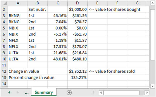
Excerpts from the results sets for the second and third select statements appear in the Excel worksheet below. The first results set displays selected column values for the first and last ten rows from the second select statement. The second results set displays selected column values for all rows from the third select statement; this is possible because there are so few rows returned by the third select statement. In addition, selected Excel analytical results appear.
- Columns A through C show data that originated with the underlying time series data.
- Columns N and O display buy_price and sell_price values from the AI model. Recall that the sell_price column value from the model is really for the last row, but the AI model permits the sale of a stock on any date after the date for the buy_price and through the last sell_price.
- Column Q shows the Percent Change from the buy_price for each potential sell_price value.
- Rows 2 through 24 show values for the first and last ten rows in the first set of trade dates.
- Rows 32 through 56 show values for all rows from the second set of trade dates.
- Key analytical results are as follows.
- Column Q values in rows 2 through 24 and 32 through 56 show, respectively for the trade dates from the second and third select statements, the Percent Change between the buy_price value and prospective sell dates.
- Cells Q28 and Q60 display, respectively for the trade dates from the second and third select statements, the median percent change between the buy_price and the set of prospective sell_price values. As you can see for the NBIX symbol the results were not particularly favorable.
- The median percent change showed no difference between buy and median sell price values from the second select statement.
- The median percent change was below the buy price for trade dates from the third select statement!

Happily, for the role of the AI model as a projection tool for identifying winning buy and sell dates, the analyses yielded more positive outcomes for the other three symbols (BKNG, NFLX, and ULTA). Here’s a summary of simulated trade outcomes with all four symbols for the first and second sets of trade dates. The simulation is for purchasing $1,000 of a security at the buy price and selling the number of shares purchased at the median sell price.
- In just eight trades with two different results sets for all four symbols, the model yielded an accumulated gain of $1,352.12 for just $1,000 put at risk in each trade.
- This is equivalent to a total percent change of more than 135 percent across the eight trades.
- While some may consider the overall results impressive, there are caveats to consider. For example:
- How do you know when to trade at the median percent change?
- Will the results be dramatically different for another set of symbols?
- The change in value was -$61.70 for the NBIX symbol.
- However, the change in value for the remaining three symbols more than made up for the NBIX loss so that the overall change in value was $1,352.12 for just $1,000 put at risk in each trade.
- How can you pick symbols that are likely to yield the most favorable outcomes?
- Is there an easy way to spot symbols and trade dates that are especially likely to yield favorable outcomes?
Next Steps
There are at least four next steps for this tip.
- Review the model description and the code to make sure you understand and can apply the model.
- Run the model with the sample data illustrated in the tip to confirm you can duplicate the results.
- Try running the model with some additional symbols beyond those presented in the tip to confirm your understanding of the data management steps as well as the robustness of the model outcomes across a wider set of symbols than those reported on in the tip.
- Adapt the model’s code to your organization’s time series data and tweak the model design to achieve the goals important to your organization. For example, could your organization benefit from a model-based approach to re-ordering inventory items or a model-based resume-screening application to exclude candidates from human consideration who are obviously unfit for a position?
The download available with this tip includes four files to help you perform the next steps described above. Here’s a brief description of each file in the download.
- “programming_AI_models_with_sql.sql” contains all the T-SQL code presented in this tip.
- “underlying_data_for_programming_artificial_intelligence.csv” contains underlying time series data for the four symbols used to demonstrate the application of the model.
- “bonus_data_for_programming_artificial_intelligence.csv” contains time series data for four additional symbols besides those explicitly presented and discussed.
- “programming_AI_models.xlsx” is an Excel workbook file. You can use it as an example to layout your own results based on the time series data for the four bonus symbols or your organization’s data warehouses and/or operational data sources.

Rick Dobson is a SQL Server professional with decades of T-SQL experience that includes authoring books, running a national seminar practice, working for businesses on finance and healthcare development projects, and serving as a regular contributor to MSSQLTips.com. He has been a practicing Python developer for more than the past half decade – with a special emphasis for data visualization and ETL tasks with JSON and CSV files. His most recent professional passions include financial time series data and analyses, AI models, and statistics. If you are interested in growing your skills in any of these areas especially as they relate to financial securities, consider visiting his blog at https://securitytradinganalytics.blogspot.com/2023/12/.
- MSSQLTips Awards: Leadership (200+ tips) – 2025 | Author of the Year Contender – 2017-2024