Using T-SQL for Investing and Trading Financial Securities

By: Rick Dobson   |   Updated: 2023-07-25   |   Comments   |   Related: > TSQL

Problem

I read several articles on how to perform specific tasks for investing and trading financial securities based on strategies coded with T-SQL. Please review the beginning-to-end steps for implementing a stock trading or investment strategy. Also, show me how to evaluate which strategies generate the largest returns.

Solution

This tip presents a high-level overview of implementing and comparing alternative plans for investing in or trading a financial security. There are several specific steps in this process.

• First, you must learn to read financial historical data about securities and transfer the data to a SQL Server instance. This can equip you to evaluate strategies based on historical data patterns.
• Second, you must decide what you want to compare.
  • Perhaps the most common example of a financial security is one where a ticker represents a company, such as MSFT for Microsoft or NFLX for Netflix. Selecting historical prices for different tickers allows you to compare the stock price for one company versus another. A ticker is an abbreviation for the name of a financial security.
  • Another example is tickers for major market indexes, such as the Dow Jones Industrial Average, NASDAQ 100, and S&P 500. You can additionally track major market indexes through exchange-traded funds (ETFs). Some tickers for ETFs based on the DOW, NASDAQ 100, and the S&P 500 indexes are, respectively, DIA, QQQ, and SPY. Traders and investors can buy and sell these ETF tickers as individual stocks for a single company.
  • ETFs for major market indexes can also be leveraged. The daily return from a leveraged ETF is a ratio of the return from the underlying basket of securities in an index. Three triple-leveraged ETFs for major market indexes have tickers of UDOW, TQQQ, and SPXL, which are respectively for the DOW stocks, NASDAQ 100 stocks, and S&P 500 indexes. The leverage ratio is for a single trading day. For a succession of trading days, the return can be greater or less than the targeted leverage ratio depending on the prices of the underlying index over those days.
  • There are many other ways of segmenting financial securities for comparative performance analyses with data mining techniques.
• Finally, you can contrast the returns for different tickers over some appropriate collection of trading days, such as daily prices for tickers from their initial public offering (IPO) date through some other date, such as ten years after the IPO or year-to-date comparisons for prices from the first trading date in a year through the most recent trading date in a year. Additionally, you can use weekly, monthly, quarterly, or annual periods for contrasting returns from financial securities. Day traders track securities prices by day parts, such as five-minute intervals from the opening of trading during a trading day.

Investing is often associated with a buy-and-hold strategy. That is, a security is bought and held for an extremely long period, such as until the onset of retirement or some major cultural change (like introducing disruptive technologies), which can offer new investment opportunities to replace prior ones. Examples of disruptive technologies include desktop computers, electric vehicles, cell phones, and AI models. Investors following a buy-and-hold strategy are likely to base investment decisions on the fundamental properties of a security, such as its earnings per share and its dividends.

In contrast, traders are more likely to base trading decisions on relatively short-term price trends. Trading is associated with buying a security and holding it until some indicator points to the value of selling a security. For a swing trader, a typical buy indicator might be the daily close price rising above its 20-day moving average. Likewise, a sell indicator might be the daily close price falling below its 10-day moving average.

Day traders hold a security over the course of a single trading day. They buy a security when the market shows a buy signal, and they sell a security when the market shows a sell signal or until sometime towards the end of a trading day. By totally exiting the market towards the end of normal trading hours, day traders avoid the volatility associated with special events, such as government economic reports during pre-market hours and company quarterly earnings reports made outside of normal trading hours.

This tip illustrates guidelines for how to compare a buy-and-hold strategy relative to a swing trading strategy based on moving averages.

Reading Daily Stock Prices and Importing Them into a SQL Server Instance

There are many sources for obtaining stock price data, such as your stockbroker, a data vendor that sells real-time and/or historical stock data, or some special sources, such as Stooq and Yahoo Finance.

A prior MSSQLTips.com article walks through the user interfaces for downloading security price and volume data for 12 tickers from two separate website sources – Stooq and Yahoo Finance. Both of these websites provide historical price and volume data without charge. As of the time the prior tip was written, the Yahoo Finance website cleaned its data more thoroughly than Stooq. In addition, Yahoo Finance is an especially well-known financial website with many articles and YouTube videos focusing on its use. Also, some of the Stooq content is in Polish so this may represent a barrier to easy use for those who are not fluent in Polish.

There are two main steps for downloading price and volume data for financial securities. First, you specify a ticker symbol. Second, you designate start and end periods for collecting historical data. A website, such as Yahoo Finance, can transfer the requested data to the download folder on the computer issuing the request for data. Typically, there is a separate downloaded file for each ticker symbol. After downloading all the data, you can cut and paste the files to a special folder for subsequent reuse and a more dedicated storage location.

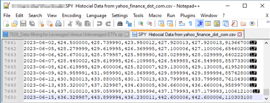
The following pair of screenshots from a Notepad++ session shows the first and last 10 rows in a CSV file for the SPY ticker symbol from Yahoo Finance; the data were downloaded on June 15, 2023. Please note these features because they will likely impact how you can use the downloaded data. For example, data is available through June 15, 2023, or earlier if the user specifies an end date before the download date.

• There are seven columns of data as denoted by the first row of column names
• Date is the value in the first column
• There are five price column names -- Open, High, Low, Close, and Adj Close
  • Price values are returned as decimal numbers with six places after the decimal point
  • The Close price is the last price during normal trading hours within a trading day
  • The Adj Close is Close price plus the prorated quarterly dividend across the trading days in a quarter
  • Traders do not typically account for dividends when tracking price performance because they seek the actual close price for a trading day
  • Investors sometimes do track Adj Close, instead of Close, to show the total returns from daily close price changes plus quarterly dividends
• The last column is for the number of shares exchanged between buyers and sellers during normal trading hours (9:30 AM through 4:00 PM Eastern Standard Time) on a trading date. Traders sometimes assign more significance to trading periods with above average volume relative to other periods
• From a data processing perspective, an essential item is that lines from Yahoo Finance end with just a linefeed (LF) instead of a linefeed plus a carriage return (LFCR), as is common for Microsoft CSV files. The referenced prior MSSQLTips.com article illustrates and explains how to account for this non-Microsoft CSV file format when bulk inserting the CSV file from Yahoo Finance to a SQL Server table
• If you elect to store the data from multiple CSV files with one file per ticker symbol in a single SQL Server table, you should also add a symbol column to the imported date, price, and volume columns. Again, the referenced prior MSSQLTips.com article illustrates how to perform this layout transformation

The following T-SQL script presents a simplified example of how to transfer the data downloaded from Yahoo Finance to a SQL Server table. This simplified example also illustrates how to download CSV file data for rows ending with a linefeed instead of a linefeed plus a carriage return.

• Two temp tables are used in the example
  • #temp_ohlcv_values is used for holding the data as downloaded by Yahoo Finance
  • #yahoo_finance_ohlcv_values_with_symbol is used for storing the data after some common data processing steps, including the adding and populating of a symbol column
• The bulk insert statement shows how to copy the CSV file downloaded by Yahoo Finance to the #temp_ohlcv_values table
  • Notice that the bulk insert statement specifies a file from the download_for_this_tip folder on the E drive as its source. This is because the downloaded data was copied from the download folder to a folder on the E drive. You can use any other destination you prefer for the copied downloaded data
  • Also, notice the ROWTERMINATOR = '0x0a' setting; this setting configures bulk insert to process files with just a linefeed signaling the end of a data row
• The select statement after the bulk insert statement echoes the data as downloaded and imported into SQL Server
• The following code segment handles the processing of the downloaded data for use in a SQL Server application
  • One column is omitted (adj close)
  • A new column is added for the security’s ticker symbol value (SPY)
• The final select statement displays the processed data

-- create two tables for importing downloaded data
-- from Yahoo Finance into SQL tables
 
drop table if exists #temp_ohlcv_values;
 
create table #temp_ohlcv_values(
 date date
,[open] money
,high money
,low money
,[close] money
,[adj close] money
,volume bigint
)
go
 
drop table if exists #yahoo_finance_ohlcv_values_with_symbol
 
create table #yahoo_finance_ohlcv_values_with_symbol(
 symbol nvarchar(10)
,date date
,[open] money
,high money
,low money
,[close] money
,volume bigint
)
 
 
-- next, do a bulk insert
bulk insert #temp_ohlcv_values
from 'E:\download_for_this_tip\SPY Historical Data from yahoo_finance_dot_com.csv'
with (
   FIELDTERMINATOR = ',', 
   FIRSTROW = 2,
   ROWTERMINATOR = '0x0a'
);
 
-- echo the data as downloaded
select * from #temp_ohlcv_values
 
-- then, process the downloaded data
-- to add a column identifying the ticker
-- symbol for a set or prices and omit columns
-- you do not want to retain (adj close)
declare @symbol nvarchar(10) = 'SPY'
 
-- insert #temp_ohlcv_values into #yahoo_finance_ohlcv_values_with_symbol#yahoo_finance_ohlcv_values_with_symbol#yahoo_finance_ohlcv_values_with_symbol
-- and populate symbol from @symbol
insert #yahoo_finance_ohlcv_values_with_symbol
select @symbol symbol, *
from
 (
  select [date]
        ,[open]
        ,[high]
        ,[low]
        ,[close]
        ,[volume]
  from #temp_ohlcv_values
 ) for_yahoo_finance_ohlcv_values_with_symbol
 
-- echo the processed data ordered by date
select   * 
from #yahoo_finance_ohlcv_values_with_symbol
order by date

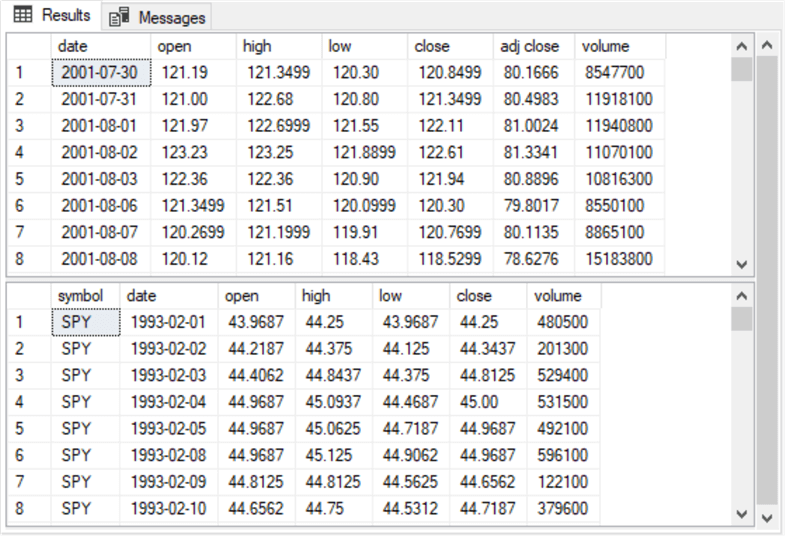
Here are excerpts from the results sets from the preceding script.

• The top window pane shows the first eight lines from the initial select statement
• The bottom window pane shows the first eight lines from the last select statement
• The inclusion of an order by clause in the last select statement accounts for the difference in displayed rows between the two select statements

Buy-and-Hold Strategies

As mentioned above, a buy-and-hold strategy is typically used by investors as opposed to traders. For this kind of strategy to result in investor success, the securities that are bought and held should have rising prices over the long run, even if the securities do experience occasional price downturns.

The Solution section of this tip highlights two types of ETFs (leveraged and unleveraged) based on major market indexes. Major market indexes in the US have increased at a healthy pace for decades, even though they have experienced occasional downturns. Within the last two to three decades, ETFs for major market indexes have become popular among some investors. Because the underlying indexes remain strong and robust over the long run, the ETFs based on the indexes are good candidates for a buy-and-hold strategy.

Investing in an ETF for a major market index is not like investing in a security for an individual company. This is because the market indexes can add and drop individual company ticker symbols at regular re-balancing times and between regular re-balancing times. When a security fails to meet the criteria for continued membership in an index, it can be dropped. Similarly, a security can be dropped from an index even if its earnings are sufficient for membership if another non-member security yields substantially superior performance.

The Solution section introduces leveraged versus unleveraged ETFs. A leveraged ETF can move a ratio of the underlying index on a daily basis. If the index goes up 2% on a trading day, then a three times leveraged ETF based on the index goes up 6%. However, if the index goes down 2%, then a three times leveraged ETF based on the index goes down 6%. If the major market indexes rise more than they decline in the long run, then leveraged ETFs are good candidates for buy-and-hold strategies because the leverage multiplies the gains from an increasing time series of prices.

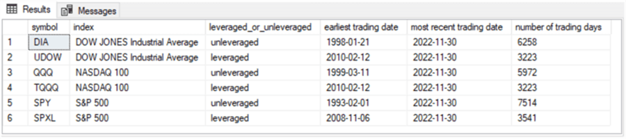
A second prior MSSQLTips.com article compares three pairs of securities based on leveraged (UDOW, SPXL, TQQQ) versus unleveraged (DIA, SPY, QQQ) ETFs. Data mining is a data science technique that offers a framework for comparing securities performance, such as assessing the comparative performance of leveraged versus unleveraged securities. You can also use data mining for various other business metrics, such as sales by branch office or time between the need to replace light bulbs of different types.

Here is a summary presented from the article that shows the ticker symbol for each ETF, the underlying index, whether the ETF is leveraged or not, the earliest trading date, the most recent trading date with price data, and the number of trading days from its earliest trading date with price data through its most recent date as of when data were collected for the article. The start date for each ticker can be different because different ETF tickers were not initially offered for sale on the same date.

The Performance Summary table below displays three performance metric values from the article reporting data mining outcomes for the buy-and-hold strategy versus a buy-sell strategy. Each of the last six columns in the second row of the table shows a ticker as a column header. The bottom three rows show the names of each of the three metrics:

• Avg % Change for the average percentage change from one trading day to the next across all the trading days for a ticker
• Performance is the name of a metric that reflects the value of the current price per share relative to the final price per share
• CAGR shows the compound annual growth rate across all the years of tracked data for a ticker

The most widely used metric for comparing different investments is the CAGR. The CAGR is the average annual growth rate across all the years an investment is held. The number of years of data for each ticker is its total trading days divided by 252 days, the approximate number of trading days in a year. The CAGR is based on the ticker in a pair with the smallest number of trading years. The tickers in a pair are the tickers for the leveraged and unleveraged ETFs for a major market index.

• The smallest number of trading years for the DIA and UDOW tickers is 12.79
• The smallest number of trading years for the SPY and SPXL tickers is 14.05
• The smallest number of trading years for the QQQ and TQQQ tickers is 12.79

As the cells in the bottom row of the following table show, the CAGR is systematically larger for each leveraged ticker (UDOW, SPXL, TQQQ) versus its corresponding unleveraged ticker (DIA, SPY, QQQ). For example,

• The UDOW ticker has a CAGR of 26.31% per year versus a CAGR of just 10.09% for the DIA ticker
• The SPXL ticker has a CAGR of 24.19% per year versus a CAGR of just 11.28% per year for the SPY ticker
• The TQQQ ticker has a CAGR of 36.65% per year versus a CAGR of just 16.04% per year for the QQQ ticker

This analysis confirms that the average annual growth rate is more than two times as large for leveraged ETFs as for matching unleveraged ETFs. Also, the TQQQ ticker, which is for large technology companies such as Microsoft, Google, and Nvidia, is dramatically larger than the other two leveraged tickers (UDOW and SPXL).

In planning your investment strategy and the associated fund’s availability, you should consider that the CAGR interest rate does not guarantee the same return for each year a security is held. In some years, it is possible for a loss to occur, while in other years, the gains may be so much larger as to more than offset the losses in other years when reporting results across all years.

The MSSQLTips.com article with excerpted results for this section of the current tip has T-SQL code for computing the three metrics to evaluate the relative market performance of unleveraged ETFs versus leveraged ETFs for major market indexes.

Computing and Using Exponential Moving Averages for Time Series Data

Financial securities analytics depend heavily on indicators. For example, the preceding section compares leveraged versus unleveraged ETFs based on three major market indexes. The purpose of the comparison is to assess if leveraged or unleveraged ETFs generated better returns. Based on the CAGR indicator, the answer for the dates and securities examined in the prior section is that leveraged ETFs generated vastly superior returns than unleveraged ETFs.

Exponential moving averages are among the most commonly used financial indicators for financial securities analytics. Exponential moving averages are weighted averages that can smooth a series of time series values over successive periods and make it easier to identify trends over time. An exponential moving average assigns two different weights to the current period’s value and the prior period’s moving average. The sum of the two weighted values is the exponential moving average for the current period. The following equation represents this relationship.

• Alpha is the weight for the current period’s value
• (1- alpha) is the weight for the prior period’s exponential moving average (ema)
• Alpha is greater than 0 and less than 1, so the current period’s exponential moving average is always a blend of two weighted values

Current_period_ema = alpha*current_period_value  + (1-alpha)*prior_period_ema

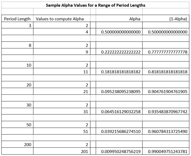
The value of alpha depends on the period length for the exponential moving average. Any one period in a time series can have one or more exponential moving averages with different period lengths. The longer the period length for an exponential moving average, the greater the degree of smoothing. The following table shows sample values of alpha and (1-alpha) for different period lengths in financial security applications. In other areas, such as engineering, different approaches may be taken to computing alpha.

There is never an exponentially smoothed value for the first period in a time series because this period does not have a prior period.

• After the initial period’s null value for the first period’s exponential moving average value, the method in this tip sets the second period’s moving average to the initial period’s value
• Other approaches wait until the tenth or a later period and base the next period’s exponential moving average equal to the average of the first ten or a larger period number of values
• The expression for computing exponential moving averages is iterative, so exponential moving average values converge in the long run towards a common value no matter for what period the first exponential moving average is computed
• On the other hand, it should be understood that starting periods are an important consideration when comparing exponential moving average values based on different starting values. The exponential moving average for any subsequent period from the starting period depends on the date and value of the initial period. Therefore, exponential moving averages with different starting periods should not be expected to equal each other for any particular date after the starting period

This tip recommends using either of two different stored procedures for computing exponential moving averages for financial applications.

• One stored procedure (usp_ema_computer) stores monetary values with the SQL Server money data type. This stored procedure is recommended where minimization of storage and fast performance are more important than the accuracy of computed values
• The other stored procedure (usp_ema_computer_with_dec_vals) stores monetary values with the SQL Server dec(19,4) data type. This stored procedure is recommended when accuracy is of the utmost importance and/or you are dividing exponential moving average values by another value
• See a prior tip titled "Money and Decimal Data Types for Monetary Values with SQL Server" for a more extended discussion of why and when to use decimal data types or money data types when processing monetary values
• Both stored procedures are in the download for this tip
  • The process for applying the usp_ema_computer stored procedure is described and demonstrated in this prior tip ("Exponential Moving Average Calculation in SQL Server")
  • The process for applying and the script for the usp_ema_computer_with_dec_vals stored procedure appears in this prior tip ("Adding a Buy-Sell Model to a Buy-and-Hold Model with T-SQL")

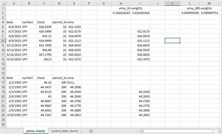
Here is an Excel spreadsheet that shows the application of the usp_ema_computer stored procedure to data downloaded and imported from Yahoo Finance in the "Reading daily stock prices and importing them into a SQL Server instance" section of this tip. The two results set excerpts in columns A through E are from applying the stored procedure for two different period lengths.

• The data in rows 5 through 12 are for a period length of 10. The date range for these rows is from the end of the results set with dates starting on 6/6/2023 and extending through 6/15/2023
• The data in rows 17 through 24 are for a period length of 200. The date range for these rows is from the beginning of the excerpted data for a date range beginning on 2/1/1993 through 2/10/1993
• The alpha and 1-alpha weight values for emas with a period length of 10 are in row 2 of columns H and I
• The alpha and 1-alpha weight values for emas with a period length of 200 appear in rows 2 of columns L and M
• The values in column I are unit test values that were computed from within the spreadsheet based on the weights along with the downloaded close and ema values returned from running the usp_ema_computer stored procedure
• An inspection of the column I values versus the column E values confirms that ema values computed and returned from the usp_ema_computer stored procedure and the computed expressions in the Excel spreadsheet match each other after rounding to four places after the decimal point

The unit test spreadsheet for the excerpts from the usp_ema_computer_with_dec_vals stored procedure shows the same values as for the usp_ema_computer stored procedure. In other words, for this application, there is no advantage to using the decimal data type versus the money data type for monetary values. However, additional downstream computations with exponential moving averages may benefit from the improved precision and rounding associated with results from the usp_ema_computer_with_dec_vals stored procedure.

Here is the SQL code for invoking the usp_ema_computer stored procedure for the SPY ticker with period lengths of 10 and 200. The data on which to compute the exponential moving averages need to be saved in a fresh copy of the yahoo_finance_ohlcv_values_with_symbol table before invoking the procedure.

-- run with a period length of 10
exec DataScience.dbo.usp_ema_computer 'SPY', 10, 0.181818181818182
 
-- run with a period length of 200
exec DataScience.dbo.usp_ema_computer 'SPY', 200, 0.009950248756219

Here is the SQL code for invoking the usp_ema_computer_with_dec_vals stored procedure for the SPY ticker with period lengths of 10 and 200. The data on which to compute the exponential moving averages need to be saved in a fresh copy of the symbol_date table before invoking the procedure.

-- run with a period length of 10
exec DataScience.dbo.usp_ema_computer_with_dec_vals 'SPY', 10, 0.181818181818182
 
 
-- run with a period length of 200
exec DataScience.dbo.usp_ema_computer_with_dec_vals 'SPY', 200, 0.009950248756219

Using a Buy-Sell Strategy for Investing in Leveraged Versus Unleveraged ETFs

The second section of this tip evaluates a buy-and-hold strategy for making gains in stock market transactions. The buy-and-hold strategy means buying a security at one date and just holding it until some distant date, such as when a newborn baby ages to the point that it is time to go to college or when an individual retires and stops working.

The second section of this tip reviews the results of a prior tip that used a data mining strategy for comparing two different sets of three securities for a buy-and-hold strategy. The data mining confirmed that leveraged ETFs (UDOW, SPXL, TQQQ) based on the three major market indexes of the DOW, S&P 500, and NASDAQ-100 indexes substantially and consistently outperformed unleveraged ETFs (DIA, SPY, QQQ) for the same three underlying indexes.

A different prior tip ("Adding a Buy-Sell Model to a Buy-and-Hold Model with T-SQL"), whose results are examined in this section, investigates if a buy-sell strategy can substantially improve the performance of the six securities examined in the second section. The buy-sell strategy is based on exponential moving averages computed with the usp_ema_computer_with_dec_vals stored procedure in the third section of this tip. In particular, four exponential moving averages (emas) with different period lengths are examined. These emas have period lengths of 10, 30, 50, and 200, where a period is equal to one trading day. The model assumes that performances for the underlying prices improve more when each ema period length is larger than an ema with the next largest period length.

In the context of the prior tip, if

• ema_10 > ema_30 and
• ema_30 > ema_50 and
• ema_50 > ema_200,

then the underlying prices for a financial security are rising. This means it is a good time to buy or hold the financial security. Otherwise, it is not a good time to buy or hold the financial security.

The strategy looks back four periods to qualify a fifth period as a good time to buy or sell a security. The T-SQL code within the prior tip referenced in this section shows when to buy and sell a security based on the following criteria.

• Two consecutive periods when it is not a good time to buy followed by two other consecutive periods when it is a good time to buy, point to setting a buy signal for the open of the fifth period
• Conversely, two consecutive periods when it is a good time to buy followed by two consecutive periods when it is not a good time to buy point to setting a sell signal for the open of the fifth period
• The first sell signal preceded by a buy signal denotes the end of the first buy-sell cycle
• Other buy-sell cycles trailing the first buy-sell cycle consists of a buy signal followed by a sell signal.
• If a sell signal occurs without a preceding buy signal, it is discarded. Likewise, it is discarded if a buy signal occurs without a trailing sell signal. Either of these outcomes is for orphaned signals within the timeframe for which a buy-sell strategy is evaluated.

Additional code within the referenced prior tip for this section keeps track of the gains and/or losses for successive buy-sell cycles in the evaluation timeframe. The sum of the gains and/or losses across the buy-sell cycles indicates the total change in a security’s value from the first buy-sell cycle to the last. The code in the referenced tip for this section uses total change values for a symbol in the evaluation timeframe to compute CAGR values.

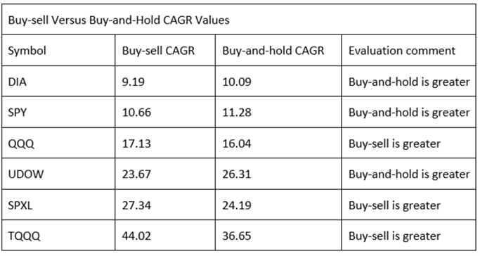
• Both buy-and-hold and buy-sell strategies have the same pattern of returning greater values for leveraged versus unleveraged securities; CAGR values for leveraged securities are consistently greater than CAGR values for unleveraged securities
• However, the buy-sell strategy does not consistently nor substantially outperform the buy-and-hold strategy
  • For three symbols (QQQ, SPXL, TQQQ), the buy-sell strategy has better performance. For three other symbols (DIA, SPY, UDOW), the buy-and-hold strategy is better
  • In addition, the median CAGR value across all six symbols for the buy-sell strategy is just about equal to the median CAGR value buy-and-hold strategy
• The relative efficacy of the buy-sell strategy versus the buy-and-hold strategy as well as the leveraged versus unleveraged securities may well merit further investigation with different ticker symbols and different timeframes before drawing any broad general conclusions
• However, for the tickers and timeframes evaluated in this tip, the conclusions appear valid

Next Steps

Before diving into the next steps from this tip, it is important to point out that this tip is not about recommending one set of tickers over another or an investing strategy over a trading strategy. This tip is an overview of selective techniques that SQL Server professionals who use T-SQL to learn about some data.

• For example, importing CSV files into SQL Server tables is a general process that can enable you to import many different kinds of data – not just financial securities data
• Also, data mining is a relatively simple data science methodology that can be configured in many different ways to find out about all kinds of data
• While moving averages are extensively used for financial securities analysis and modeling, exponential moving averages can be used in many different contexts. I once worked at the largest nuclear power generation plant in North America during a time when there were many engineering changes being made at the plant. Moving averages were computed to verify the status of compliance with regulatory rules for the status and ultimate completion of these changes

I hope some readers will adopt my enthusiasm for performing financial securities modeling. As you can see from the range of topics addressed in this tip and the bullet points below, financial securities modeling is a very broad topic.

• When starting to learn and practice financial securities modeling, pay special attention to data mining for any subset of financial security topics that interests you
• I started years ago by focusing on financial securities indicators and importing financial securities data into SQL Server. Examine my prior tip titles for a starter sample of financial security topics that you may find fruitful for investigating with your SQL Server skills
• Also, consider reading good tutorial articles on financial securities analysis. I find Investopedia a good source for quick, clear reads about a broad range of financial topics. StockCharts.com is another excellent source for learning about financial securities indicators and, of course, stock charts; a special advantage of SQL Server is that you can go beyond charts to more rigorous forms of analysis than is possible with charts. Once you know what financial topics you want to learn more about, the Wikipedia website may prove to be a valuable place to visit
• As you might be able to tell from this article, I am particularly excited about using SQL Server to predict when it is time to buy, hold, and sell securities. This kind of interest is especially appropriate for those who want to become skilled traders
• You do not have to invest or trade financial securities to test your skills in investing or trading financial securities. All you need is historical stock price data and a lot of imagination about anticipating price upturns and downturns. This tip can get you started for importing stock price data into SQL Server
• Finally, if you start investing or trading financial securities and you get rich, please do not blame me. The credit and the rewards will be all yours

About the author

Rick Dobson is an author and an individual trader. He is also a SQL Server professional with decades of T-SQL experience that includes authoring books, running a national seminar practice, working for businesses on finance and healthcare development projects, and serving as a regular contributor to MSSQLTips.com. He has been growing his Python skills for more than the past half decade -- especially for data visualization and ETL tasks with JSON and CSV files. His most recent professional passions include financial time series data and analyses, AI models, and statistics. He believes the proper application of these skills can help traders and investors to make more profitable decisions.

This author pledges the content of this article is based on professional experience and not AI generated.

View all my tips