By: Levi Masonde | Updated: 2023-10-26 | Comments | Related: > Python
Problem
Suppose you are a data scientist for an insurance company looking to predict the life expectancy of a particular country for the next five to eight years, along with how much a region spends on its healthcare and population. How can you use machine learning to make these predictions?
Solution
You can use Python's machine learning library, TensorFlow, to make future predictions on life expectancy. Even if you have never used Python, this tutorial aims to help absolute beginners and experienced users the same. To be more specific, this tutorial will focus on supervised machine learning.
Supervised machine learning algorithms are mainly used when the output is classified or labeled. In this instance, we can use analysis and regression to predict the life expectancy for a country using specific parameters.
Set Up Your Environment
The prerequisites for this tutorial include:
- Windows 10
- Visual Studio Code
- Python 10.9
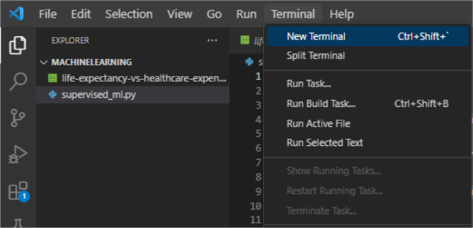
Once all the prerequisites are set, open Visual Studio Code, click the Terminal tab, and click New Terminal to start a new terminal:

On the new terminal, use Python's pip to install pandas, matplotlib, and sklearn:
pip install pandas matplotlib scikit-learn
Loading the Dataset
Supervised machine learning relies on data input, also known as training data. The aim here is to train or feed the algorithm with the input data and the expected output data; this will enable the algorithm to essentially build its own logic of how to get from the given input data to the expected output. The more input data is fed to the algorithm, the better the results will be since the training will cover a lot of cases.
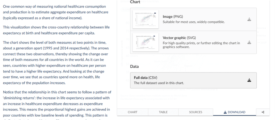
This tutorial will use life expectancy data from Our World In Data. Click the download tab and the Full Data (CSV) file button to download the relevant data.

After downloading the data, place the CSV file in your project directory to gain easy access.
Summarizing the Dataset
Supervised learning algorithms usually try to link two datasets and learn how they relate. There is the observed data X and an external variable y that we are trying to predict called "target" or "labels." y is usually a 1D array of length n samples.
This tutorial will use the scikit-learn module to fit our life expectancy model and predict how life expectancy and healthcare will grow in the future for various countries.
All supervised estimators in scikit-learn implement a fit (X, y) method to fit the model and a predict(X) method that, given unlabeled observations X, returns the predicted labels y.
Let's start coding. Start by creating a Python file named supervised_ml.py.
Since you already have the CSV file in your project folder, you can use this code to retrieve the data and store it in a dataframe:
import pandas as pd
import numpy as np
import matplotlib.pyplot as plt
from sklearn.model_selection import train_test_split
from sklearn.linear_model import LinearRegression
from sklearn.metrics import mean_squared_error, r2_score

# Load the dataset
data = pd.read_csv("life-expectancy-vs-healthcare-expenditure.csv")
Visualizing the Dataset
While the above code fetches data, looking at the data you are about to process is always a good idea. This will help you evaluate and process data better with a clear understanding of how to manipulate the data. To view your dataset, add the following code to your supervised_ml.py:
print(data)
To run your code, click the play button at the top right corner of Visual Studio Code, which should show the dataframe structure:

Now that we have confirmed the collected data, let's use our installed Python libraries to evaluate the data. We will use the Mean Squared Error (MSE) and R-squared (R^2) metrics to evaluate the regression models' performance.
MSE measures the average squared difference between the actual values (ground truth) and the predicted values produced by a regression model. The smaller the MSE, the better.
R^2 measures the proportion of the variance in the dependent variable (target) explained by the independent variables (features) in the regression model. The R^2 is a value between 0 and 1, where 0 indicates that the model does not explain any variance, and 1 indicates that the model explains a larger portion of the variance.
Add the following code to the supervised_ml.py to filter the data for a set country and evaluate the data:
import pandas as pd
import numpy as np
import matplotlib.pyplot as plt
from sklearn.model_selection import train_test_split
from sklearn.linear_model import LinearRegression
from sklearn.metrics import mean_squared_error, r2_score

# Load the dataset
data = pd.read_csv("life-expectancy-vs-healthcare-expenditure.csv")

data.drop("Continent",axis=1, inplace=True)
data.drop("Code",axis=1, inplace=True)

# Drop rows with missing values
data.dropna(inplace=True)

# Filter the data for a specific country
data = data[data['Entity'] == 'France']

# Select the relevant columns
X_life_expectancy = np.asarray(data[["Year", "Life expectancy at birth, total (years)"]])
X_healthcare_costs= np.asarray(data[["Year", "Current health expenditure per capita, PPP (current international $)"]])
X_population = np.asarray(data[["Year", "Population (historical estimates)"]])
y_life_expectancy = np.asarray(data["Life expectancy at birth, total (years)"])
y_healthcare_costs = np.asarray(data["Current health expenditure per capita, PPP (current international $)"])
y_population = np.asarray(data["Population (historical estimates)"])

# Split the data into training and testing sets
X_train, X_test, y_train, y_test = train_test_split(X_life_expectancy, y_life_expectancy, test_size=0.4, random_state=25)

# Create a Linear Regression model for life expectancy
lr_life_expectancy = LinearRegression()
lr_life_expectancy.fit(X_train, y_train)

# Make predictions for life expectancy
y_pred_life_expectancy = lr_life_expectancy.predict(X_test)
predict_years = np.arange(2020, 2028)

# Evaluate the model for life expectancy
mse_life_expectancy = mean_squared_error(y_test, y_pred_life_expectancy)
r2_life_expectancy = r2_score(y_test, y_pred_life_expectancy)

# Print the evaluation metrics
print("Life Expectancy Model:")
print("Mean Squared Error:", mse_life_expectancy)
print("R-squared:", r2_life_expectancy)

# Then, split X and y_healthcare_costs using the same X_train and X_test
X_train_health, X_test_health, y_train_health, y_test_health = train_test_split(X_healthcare_costs, y_healthcare_costs,  test_size=0.4, random_state=25)

# Create a Linear Regression model for healthcare costs
lr_healthcare_costs = LinearRegression()
lr_healthcare_costs.fit(X_train_health, y_train_health)

# Make predictions for healthcare costs
y_pred_healthcare_costs = lr_healthcare_costs.predict(X_test_health)

# Evaluate the model for healthcare costs
mse_healthcare_costs = mean_squared_error(y_test_health, y_pred_healthcare_costs)
r2_healthcare_costs = r2_score( y_test_health, y_pred_healthcare_costs)

print("\nHealthcare Costs Model:")
print("Mean Squared Error:", mse_healthcare_costs)
print("R-squared:", r2_healthcare_costs)

# Then, split X and y_healthcare_costs using the same X_train and X_test
X_train_population, X_test_population, y_train_population, y_test_population = train_test_split(X_population, y_population,  test_size=0.4, random_state=25)


# Create a Linear Regression model for population
lr_population = LinearRegression()
lr_population.fit(X_train_population, y_train_population)

# Make predictions for population
y_pred_population = lr_population.predict(X_test_population)

# Evaluate the model for population
mse_population = mean_squared_error(y_test_population, y_pred_population)
r2_population = r2_score(y_test_population, y_pred_population)

print("\nPopulation Model:")
print("Mean Squared Error:", mse_population)
print("R-squared:", r2_population)
After running the code again, the code outputs the following evaluation results for our data:

Due to the high amount of data we supplied our models, it is not surprising that the models perform extremely well when evaluated.
Making Predictions
To create predictions using our models, the train_test_split() method from the sklearn.model_selection module and the predict() method from the LinearRegression method will be used, as shown in the code on the supervised_ml.py file.
To show these predictions on a graph, add the following code to the supervised_ml.py file:
# Plot the life expectancy results
plt.figure(figsize=(12, 4))
plt.subplot(1, 3, 1)
plt.plot(predict_years,y_pred_life_expectancy, color="red", linewidth=3)
plt.xlabel("Year")
plt.ylabel("life_expectancy")
plt.title("life expectancy Prediction")

# Plot the life expectancy results
plt.subplot(1, 3, 2)
plt.plot(predict_years,y_pred_healthcare_costs, color="blue", linewidth=3)
plt.xlabel("Year")
plt.ylabel("Healthcare Costs")
plt.title("Healthcare Costs Prediction")

plt.subplot(1, 3, 3)
plt.plot(predict_years, y_pred_population, color="purple", linewidth=3)
plt.xlabel("Year")
plt.ylabel("Population")
plt.title("Population Prediction")

plt.tight_layout()
plt.show()
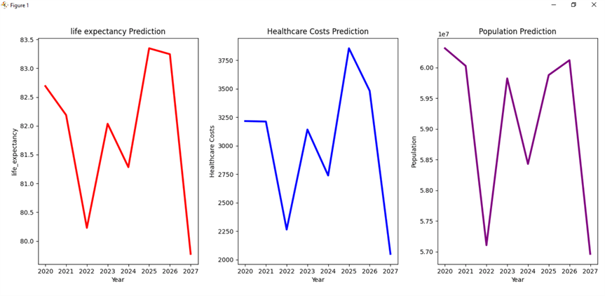
After running the code, a figure will appear with your plotted graphs next to each other. This will show you how the factors are related:

The above predictions are for the country of France. You can change the country by changing this line of code.
data = data[data['Entity'] == 'France']
Final Thoughts
The correlation of the graphs proves that the algorithm does make predictions based on all the factors included in the source data. To see how it affects the results, you can analyze the data further by changing variables, such as the test_size and random_state, on the train_test_split() method.
You should keep in mind that some of the data is missing on this dataset. To get the full scope of the data, ensure you subscribe to paid data providers with extensive data logs. This tutorial is an example of how to approach this problem or similar ones.
Next Steps
- See how ChatGPT uses Machine Learning: Large Language Models (LLMs) to train artificial intelligence (AI) tools such as ChatGPT.
- Learn how to set up your Python environment for Machine Learning: Machine Learning Services – Installation and Configuration.
- See Machine Learning examples using SQL: Classic Machine Learning Example In SQL Server Analysis Services.
- Learn how to visualize your Machine Learning data analysis: SQL Server 2017 Machine Learning Services Visualization and Data Analysis.
About the author
 Levi Masonde is a developer passionate about analyzing large datasets and creating useful information from these data. He is proficient in Python, ReactJS, and Power Platform applications. He is responsible for creating applications and managing databases as well as a lifetime student of programming and enjoys learning new technologies and how to utilize and share what he learns.
This author pledges the content of this article is based on professional experience and not AI generated.
View all my tips
Article Last Updated: 2023-10-26


