Improve Power BI Performance with Horizontal Filtering

By: Kenneth A. Omorodion   |   Comments   |   Related: 1 | 2 | 3 | > Power BI

Problem

In Part 1 and Part 2 of this series, I demonstrated how implementing Vertical Filtering, preference for custom columns created in Power Query, disabling "Auto date/time" in data load options settings and using more variables in DAX measures calculations could help improve performance of Power BI reports.

In this third part of the series, I will demonstrate how removing unnecessary rows or Horizontal Filtering and the disabling of Power Query query load for non-required tables could be used to optimize Power BI report performance. I would encourage you to read Part 1 and Part 2 of this series to ensure you understand all discussed options available for performance optimization in Power BI.

Solution

This part of the series will focus on what steps to take to configure performance optimization using Horizontal Filtering and the disabling of Power Query query load for non-required tables.

Power BI Horizontal Filtering

This is particularly useful where the model size is rather large and one would not be able to efficiently develop visuals or create calculations in Power BI without considerable impact on the speed of rendering of visuals and having very slow query performance. Horizontal Filtering is another word for limiting the number of rows in a dataset, thereby improving model performance.

It is important to note that Horizontal filtering could be achieved by loading models with filtered rowsets either by Filtering by time or Filtering by entity. However, for the purpose of this tip, I am concentrating on the former, which helps in performance optimization of slow models in Power BI. You can read more on Horizontal Filtering methods here.

Microsoft suggests that you do not automatically load all available history data, apart from cases where this is a known reporting requirement. What we are trying to achieve with this technique is ways to only load a subset of the history data into the data model thereby considerably reducing the amount of data we are working with at any particular time, thus improving speed of query refreshes and visual rendering while creating visuals. Optimally, when we finish creating the visuals and published to Power BI service, we can readjust the dataset to load full history data. This process is summarized this below.

1. Import the dataset
2. Create a parameter for the Order Date column
3. Apply the parameter to filter the Order Date column using the Custom option
4. Load the filtered dataset into the data model
5. Create visuals as needed with the reduced/filtered dataset
6. Save and Publish to Power BI Service workspace
7. Go to Power BI Service and configure gateway (if required), Configure parameter settings, and configure schedule refresh (as needed)
8. Manually refresh the dataset

Step 1: Import the dataset

Okay, we know what we want to achieve now and what steps to follow to achieve it, so let's see how this is done.

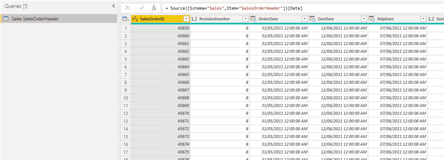
I am using the SalesOrderHeader dataset imported from AdventureworksDB2014. This is just for illustration purposes; any other dataset can be adapted for this technique. The three diagrams below show how I have imported the dataset into Power BI Desktop.

Then select the table you require as shown below.

The table is now in Power Query Editor in Power BI Desktop as seen below.

Step 2: Create a parameter for the Order Date column

Next step is to create a parameter to hold a date value for use in filtering.

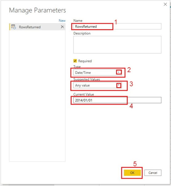
The diagram below shows how to configure the parameter. Just give the parameter a name, I called mine RowsReturned. You can give a description for it but its optional. Then you need to select a data type, so I selected "Date/Time" since I am planning to filter on a date column. For "Suggested Values" choose "Any value". For "Current Value" I just choose a date value existing in the OrderDate column of the dataset. Learn more about creating Query Parameters here.

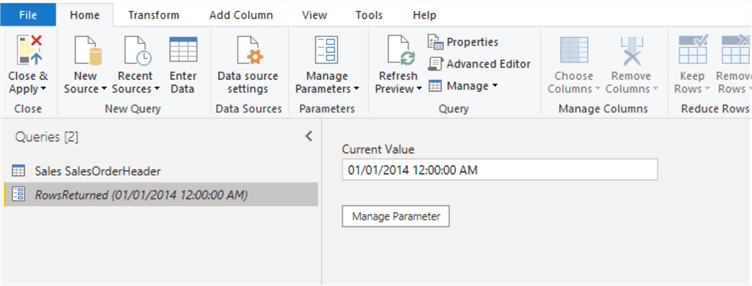
After creating the parameter, it should look like the diagram below.

Step 3: Apply the parameter to filter the Order Date column using the Custom option

Now it's time for us to apply the created parameter to the OrderDate column for filtering. Before doing this, you can quickly check how many rows your dataset currently has, in my case it was about 31,465 rows before filtering. I have used the OrderDate column in this tip, you can choose to use any other date column as required. See the following diagrams for how this is done.

In the diagram below, I have selected the "Custom Filter" option for configuring the filtering with the parameter created earlier.

The next diagram below shows the dialog box to enter the filter conditions. So, I have entered "is after or equal to" on the "Keep rows where OrderDate''‘. You can use any other selections like "is before or equal to", this really depends on your business need. But, for the purpose of this tip, I wanted to choose a date within my OrderDate values to eradicate chances of issues. Then, I further selected "Parameter" from the date dropdown. This is the parameter I created earlier with value of "01/01/2014". Note that I have not entered anything on the selection box below the top ones, but you can adapt that aspect to your business need to further provide filtering conditions.

Step 4: Load the filtered dataset into the data model

Next step is to load the already filtered dataset into the data model and verify number of rows now loaded. Click "Close & Apply" to load the model. As can be seen in the diagram below, my dataset now has only 11,761 rows (from an initial 31,465). This can be more efficient when applied to larger datasets with millions of rows drastically reducing the size of the data to work with.

Step 5: Create visuals as needed with the filtered dataset

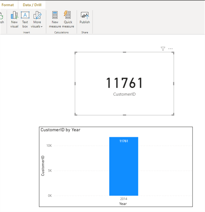
For this tip, I am not going to dwell much on how to create visuals, but I have created a column chart showing total customers by year. This currently is showing only 2014 for year in accordance with our filter condition applied earlier. See diagram below.

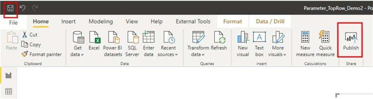
Step 6: Save and Publish to Power BI Service

Next is to save the work and publish the report/dataset to Power BI Service workspace as seen in the diagram below.

Step 7: Configure Power BI gateway, parameter settings, and schedule refresh

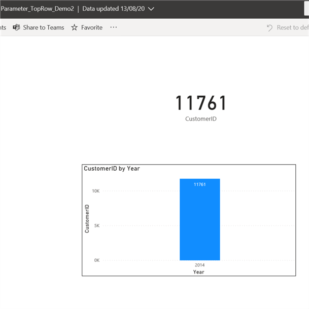
Next step is to configure the parameter settings in Power BI Service. Before doing this try to view what is currently showing on the report, it should be exactly what you have created in Power BI Desktop with only 2014 data in this instance as shown below.

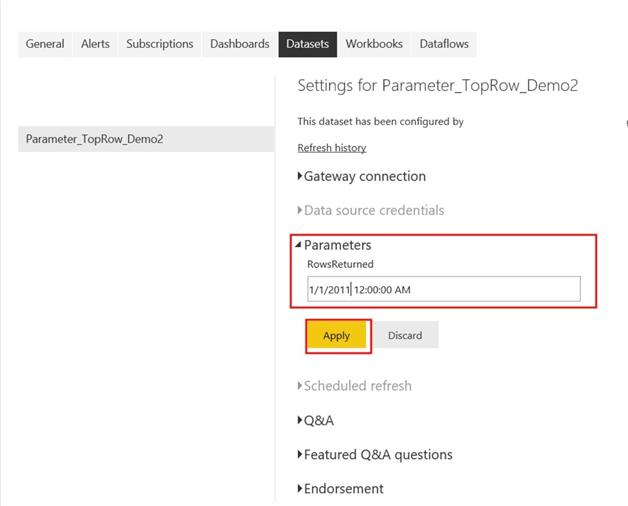
Then, let's go configure the Parameter settings so we can override the filtering and load all history data and get all 31,465 rows again. This is as seen in diagrams below.

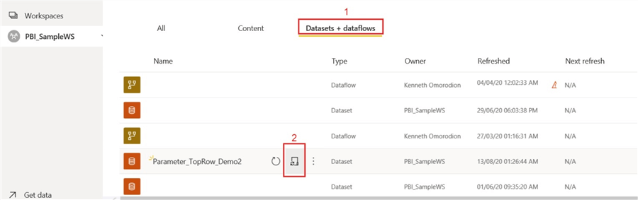
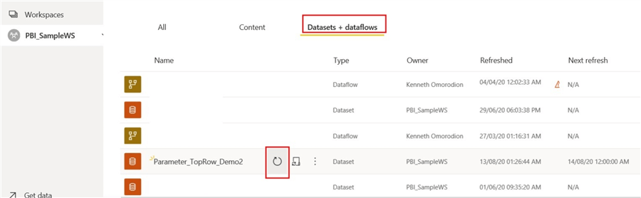
Click on "Datasets & Dataflows". Then, click on "schedule refresh" icon

Initially, when you get to the Parameter settings as seen on the diagram below, it would have the default date applied for filtering (i.e. 2014/01/01).

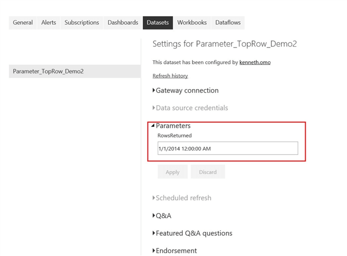
We need to now change this as far back as when the historical data started. In this case its 2011 May, but I will just start from 2011/01/01 (this was the reason we used "is after or equal to" earlier"). This is shown in the diagram below.

Next, we need to configure the gateway to recognize the data source, if this is not already done. You can learn more about how to configure a data source with an On-Premises data gateway here.. You might also need to configure the schedule refresh to ensure your dataset refresh without issues later. See one of my tips which demonstrate how to configure schedule refresh.

Step 8: Manually refresh the dataset

After these, the next step is to go back to "Datasets & Dataflows" as seen below to carry out a one-off manual refresh of the dataset.

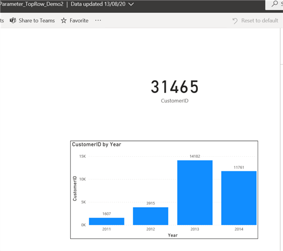
After this go back to the report view and verify the number of rows that is now returned in the visuals. If your visuals are still the same, try to refresh the Power BI service page, you should be able to now see that the number of rows is 31,465 and that there is now more Years than just 2014 as seen below.

Disabling of Power Query query load for non-required tables

Every single query loaded into the data model leads to memory consumption. However, as we have seen in most of the techniques in this optimization series, the main asset has largely been memory conservation. The higher the memory consumed, the higher the likelihood of negative performance impact on the model. Thus, it is good practice to disable un-required queries to improve performance.

It is also important to understand that when a query is disabled to load into the data model, it is only not loaded into the memory, but the query still refreshes as usual. To demonstrate this, I have imported two datasets holding Employees details for 2008 and 2009. Both tables have the same columns but different number of rows. So, we can append the tables. To ensure this tip is brief enough, I will not go into detail on how I have imported the tables or how to append datasets. However, I will demonstrate how if both the appended dataset and the individual (2008 & 2009) datasets can consume memory if all is loaded to the data model.

The diagram below shows the three datasets (the 2008, 2009 and the appended dataset known as Employees).

I will now click on "Close & Apply" to load all datasets to the memory so we can see the memory consumed as seen in the diagram below.

As can be seen in the diagram above, the current memory used up by the data model is about 232KB (but imagine if this was a very large model). Then let us go back to Power Query Editor and disable the load of the individual datasets (Emp_2008 & Emp_2009) so we can tell if the memory usage has increased or decreased. So, as seen in the diagram below, we need to right click on both datasets individually (Emp_2008 & Emp_2009) and un-check the checked box at the front. This would ensure the data load is disabled for each dataset leaving us with only the appended (Employees) dataset to be loaded into memory. Note you will see the font type of the load disabled datasets change to italics.

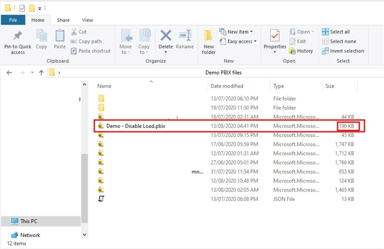
Then click "Close & Apply" to load the Employees table only to the data model. After this we can verify that we have saved memory by disabling the load of two datasets not required in the model individually as seen in the diagram below. The memory consumption is now about 196KB from the initial 232KB (a difference of about 36KB). Again, imagine if this were a massive model, this could have made a difference.

Next Steps

• See the first part of this series of improving performance of Power BI model
• See the second part of this series of improving performance of Power BI model
• Try this tip out in your own data as needed

Learn more about Power BI in this 3 hour training course.

About the author

Kenneth A. Omorodion is a Business Intelligence Developer with over eight years of experience. He holds both a bachelor’s and master’s degree (Middlesex University in London). Kenneth has the MCSA, Microsoft Data Analyst - Power BI and Azure Fundamentals certifications. Kenneth is a Microsoft Certified Trainer and has delivered corporate training on Power BI, SQL Server, Excel and SSRS.

This author pledges the content of this article is based on professional experience and not AI generated.

View all my tips