Comparing with T-SQL and Excel a Decision Tree Regression to a Bagged Regression

By: Rick Dobson   |   Comments   |   Related: > TSQL

Problem

Please present comparisons of a decision tree regression versus a bagging regression based on two different test datasets. Demonstrate how to perform the comparison using both T-SQL and Excel.

Solution

Each of the two prior tips illustrate the mechanics of how to implement two different data science models for the same source data. This prior tip demonstrates how to build a decision tree regression model with T-SQL. The other prior tip, Multiple Regression Model Enhanced with Bagging, illustrates how to build a bagged regression model with T-SQL code based on the same source data in the prior tip. These two data science models are also commonly referred to as machine learning models.

Both decision tree regression models and bagged regression models can account for the variance of target column values based on two or more predictor column values. Decision tree regression takes multiple columns of potential predictor variables and finds a subset of predictor columns that best account for the variance of the target column values. Bagged regression assumes a basic model structure, such as the one developed in a prior decision tree regression. Then, it divides the source data into several bags or groups and fits the same assumed model structure to each bag of data. Finally, bagged regression aggregates the model estimates for each bag of data into one overall model. While decision tree regression builds one model from all the source data, bagged regression builds an overall model based on multiple sets of bagged rows from the original source dataset rows.

This tip uses T-SQL and a SQL Server database to manage the output associated with each type of model. Routine data wrangling tasks shape the output from each model type for comparative purposes. Next, the SQL Server data is copied and pasted into Excel for the implementation of the comparison. This tip provides a demonstration of data science concepts such as cross validation, model variance, and model bias. The download for this tip includes T-SQL source code along with sample data tables for data wrangling as well as an Excel workbook to demonstrate the expressions used to implement the model comparisons. This tip is different than nearly all other internet resources on machine learning in that it explains, demonstrates, and compares machine learning models with T-SQL code and Excel worksheets.

An overview of the decision tree regression and bagging regression models

The following diagram (Decision Tree Regression Without Bagging) is populated with values based on the initial prior tip which demonstrates how to implement a decision tree regression. A decision tree regression uses each row from the source dataset just once. Each node in the decision tree corresponds to a set of rows from the source data.

• For example, this tip's source dataset for the decision tree regression is based on a dataset with 294 rows.
  • The top node, commonly called a root node, of the decision tree corresponds to all the rows in the source dataset.
  • The target column values are average daily snowfall in inches during a quarter of the year. From all 294 weather observations, there is an average daily snowfall of .0965 inches.
  • Decision tree regression models segment dataset rows based on predictor columns category values. Then, the decision tree regression model algorithm searches successively for predictor columns that best account for the variance of values in the target column at each level of the decision tree.
  • For the data in the initial prior tip, two predictor columns were found to optimally account for target values:
    • The first predictor is the longitude of the weather station from which the snowfall was recorded
    • The other predictor is type of quarter (wintery or non_wintery) when the snowfall was recorded.
  • Weather observations were made for the quarters of the years 2016 through 2019.
• Directly below the root node there are three more nodes with titles of we_east_indicator rows (for weather observations form New York), we_middle_indicator rows (for weather observations from Illinois), and we_west_indicator rows (for weather observations from Texas).
  • Notice that the sum of the counts for the three nodes below the root node is 294 (97 + 89 +108).
  • This outcome confirms that these three nodes segment the rows in the root node.
• The bottom node in each path through a decision tree is called a leaf node. Any node with one or more nodes below it is called a parent node. There are two leaf nodes for each of the three parent nodes directly below the root node.
  • One of the leaf nodes has the title wintery_quarter rows.
  • The other leaf node has the title non_wintery rows.
• The row counts for the pair of leaf nodes below each parent node sum to the row count for the parent node.
  • For example, the row count values for the leaf nodes below the we_east_indicator rows node (47 and 50) sums to 97, which is the row count value for the we_east_indicator node.
  • This confirms that each pair of leaf nodes segments the rows in its parent node.

The following diagram (Decision Tree Regression With Bagging) is for a bagged regression model. The bagged regression model is explained and demonstrated in the second prior tip Multiple Regression Model Enhanced with Bagging). While the source data for both models are the same, the source data are processed differently within each model.

• The bagged regression model is based on five bags of data rows.
  • Each bag consists of 80 rows.
  • Bag rows are selected randomly with replacement from the full set of 294 rows in the original source dataset. Because of the "with replacement" constraint, a bag may contain two or more duplicates of the same data row from the original set of 294 rows.
  • Furthermore, it is not guaranteed that all rows from the original dataset will populate the full set of bags for which rows are randomly selected.
  • Original data source rows not selected for any bag can be used for a hold-out sample to verify that bagged regression based on five bags also applies to other rows from the original population of data values. Training a model on one set of rows and testing the model on another set of rows is a common data science technique. This is sometimes called cross validation.
  • You can achieve random selection with replacement by invoking the T-SQL rand function.
• After creating 5 bags of 80 rows each, you can create a model for each bag.
  • The full set of 80 rows for each bag are for the root node of a bag.
  • Within each bag, the 80 rows are split into three sets (we_east_indicator rows, we_middle_indicator rows, and we_west_indicator rows) based on the longitudinal value of the weather station from which a weather observation is made. These three sets of rows are for each of the nodes directly below the root node for a bag.
  • Next, each of the three sets of rows are segmented into two sets for wintery_quarter rows and non_wintery quarter rows. These three pair of rowsets are for the leaf nodes within each bag.
  • By computing the average snowfall per node and the count of rows per node, you can specify a tree diagram for each bag.
• Next, you can average the count of rows per node and average snowfall per node across the five bags. The average values across the leaf nodes constitute the regression parameter estimates.

Data for this tip

There are two test datasets within this tip to compare the decision tree regression model to the bagged regression model.

• The first test dataset is the training dataset for the bagged regression model plus one additional column.
  • Recall that this dataset is comprised of five sets (or bags) or 80 rows each. Within each bag are predictor columns and an observed (or target) column.
  • There is no estimated weather observation. After all, the whole purpose of a regression model is to estimate the observed value given the predictor values.
  • However, when comparing two different regression models, it is necessary to have the estimated and observed values from both models to assess if there is a model that is better at estimating observed values.
• The second test dataset is based on the original source dataset rows that were not selected for inclusion in the bagged regression training dataset.
  • Although there are 400 rows in the bagged regression training dataset, not all the rows within a bag and certainly across bags are unique. In fact, there are just 221 unique dataset rows in the bagged regression training dataset.
  • Because there are 294 distinct rows with predictor and observed weather column values in the original data source, there are 73 data rows (294 – 221) which are not in the bagged regression training sample. These 73 rows are called the hold-out sample in this tip.
  • Similar to the bagged regression training sample, estimated values from each type of model are needed to implement the comparison of the decision tree regression model with bagged regression models across both the training sample and the hold-out sample.

Data for comparing models based on the bagged regression training set

One way to operationalize the comparison of model outputs is through assessing the correspondence between the observed target values and the estimated target values. Each model is estimated based on different data processing rules. However, both models should be compared to one another in an identical way. That means running the same set of comparative analyses for each model with respect to both the bagged regression training sample and the hold-out sample.

Because of design specifications between the two regression models, the estimated weather values can be distinct between the two models while the observed weather values are the same for both models.

• For the decision tree regression, there is a total of 294 total weather observations. The decision tree regression model returns an estimated weather observation to match each actual weather observation.
• For the bagged regression
  • There are 80 weather observations in each of 5 bags of observations. This results in a total set of 400 (80 X 5) observed values. Each of the 400 bagged observations has a row_id value that corresponds to row identifier for one of the 294 observations in the underlying source data.
  • The 400 observations across the 5 bags are aggregated based on the nodes for a decision tree. Each bag has its own set of node values for a decision tree. See the prior tip on estimating a bagged regression model for details on how to perform the aggregation.
    • The decision tree structure is the estimated decision tree based on the 294 observations for the decision tree regression. This model's structure is re-used to help estimate the bagged regression model.
    • The observed values within a bag derive from randomly selected rows with replacement from the original dataset of 294 rows.
    • The average weather across the five bags for each node in the decision tree structure is the output of estimated target values from the bagged regression model.

To compare the decision tree regression model and bagged regression model, it is desirable to have both models return results for the same set of data rows. These are 400 training set rows originally used to estimate the bagged regression model.

Excerpts from the query to return the 400 rows with the actual weather observations and the estimated weather observations for the decision tree regression appear in the next table. There are three key sources of the results set:

• A table containing 400 random numbers retuned as 5 sets of 80 rows: one set for each bag.
  • On each row is a random number (rand_digit) in the range of 1 to 294. The random numbers point at the underlying source data of 294 rows.
  • The sample_id column designates the bag number. Within this tip, the possible sample_id values extend from 1 through 5.
  • The row_id column from this table specifies a row number from 1 through 80 within each bag.
• Another table data source has a row identifier column (row_id_pt), a station identifier column (noaa_station_id), predictor columns (snowy_quarter_indicator and long_dec_degree_one_third_tile_indicator), and an observed weather column (target).
• The estimated_target_dtr column contains the estimated target values from the decision tree model based on predictor column values.

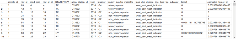
The four excerpts in the following table shows the overall structure of the model output from the decision tree regression model. This model output facilitates the comparison of the decision tree regression with the bagged regression.

• The first row of the following table contains an image of the first ten rows of model output.
  • For each row in this set, the rand_digit column values match the row_id_pt column values.
    • The rand_digit column values are from the table with 400 random numbers to enable random selection with replacement.
    • row_id_pt column values are from the data source comprised of 294 row identifier column values along with matching station identifier column values (noaa_station_id), predictor column values (snowy_quarter_indicator and long_dec_degree_one_third_tile_indicator), and observed weather column values (target).
  • The sample_id column values designate the bag number. All ten rows in the first row below are from the first bag of 80 rows.
  • The row_id column designates a row order number for the 80 rows in a bag. Therefore, row_id column values are always in the range 1 through 80.
  • The rand_digit column values are from an expression based on the T-SQL rand function that returns values in the range of 1 through 294.
  • The row_id_pt column values are from the original source data of 294 rows.
    • The row_id_pt column value from the original source data always matches the rand_digit column value from the 400 random row numbers based on sampling with replacement.
    • Some row values from the extreme left column of the Results pane, such as rows 3, 4, and 5, have the same row_id_pt value. When a row_id_pt value repeats two or more times, this is an example of the duplicated row being selected one or more times for the same bag.
    • Three duplicated row_id_pt values appears in rows 5, 24, and 76 within the first bag. These three duplicated values correspond to row numbers 3, 4, and 5 from the extreme left column of the Results pane.
    • The target column values are observed weather values. The values in this column contain the average of the observed snowfall in inches from a weather station in a quarter during a year. Quarter column values are recoded into one of two predictor column values within the snowy_quarter_indicator column.
      • Quarters 1 and 4 are recoded as wintery quarter.
      • Quarters 2 and 3 are recoded as non_wintery quarter.
    • The STATEPROV column designates the state in which a weather station resides.
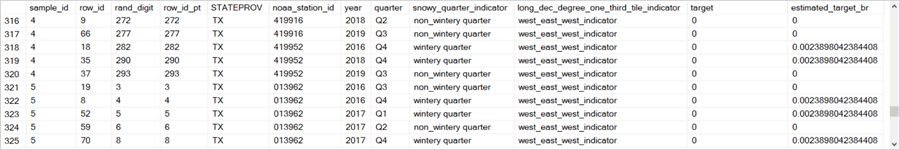
• The second image of rows in the following table contains the last five rows of the first bag trailed by the first five rows of the second bag.
  • The last five rows of the first bag all have a sample_id value of 1 – just like in the first ten rows in the following table. These five rows have row numbers of 76 through 80 in the extreme left column of the Results pane.
  • The first five rows of the second bag all have a sample_id value of 2, which points at the second bag. These five rows have row numbers of 81 through 85.
• The third image of rows in the following table contains the last five rows of the fourth bag trailed by the first five rows of the fifth bag. The sample_id values again indicate the bag number.
• The fourth row in the following table displays the last ten rows from the fifth bag. Therefore, all these rows have a sample_id of 5.

The four excerpts in the following table displays the overall structure of the model output from the bagged regression model.

• The columns from sample_id through target have the same names as for the results set excerpts from the decision tree regression model. Furthermore, the row values for these columns are the same as well.
• On the other hand, the last column name and its row values are distinct between the bagged regression and the decision tree regression results sets.
  • The last column in the following set of excerpts has the name estimated_target_br to signify that the row values are from the bagged regression model. The name of the last column in the preceding table is estimated_target_dtr to indicate that the row values are from the decision tree regression model.
  • Because the computational approach for estimating node values is different in the decision tree regression model versus the bagged regression model, the estimated_target_br column values are generally distinct from the estimated_target_dtr column values.

Data for comparing models based on the hold-out sample

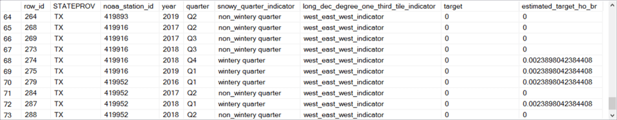
This section gives you a view of sample rows from the hold-out sample. Recall that there are just 73 rows in this sample. Also, there are two different versions of the hold-out sample.

• The first version displays decision tree regression estimated weather values in its last column (estimated_target_ho_dtr).
• The second version displays bagged regression estimated weather values in its last column (estimated_target_ho_br).

The columns preceding the last column are for identifying individual rows, predictor column values, and observed weather values.

• The row_id column contains row number values from the original set of 294 observed weather rows. There is no overlap between the row_id column values from the hold-out sample and the row_id_pt column values from the bagged regression training set.
• The snowy_quarter_indicator and long_dec_degree_one_third_tile_indicator columns contain predictor values.
• The target column contains observed weather values.
• Other columns are for reference purposes. For example, noa_station_id contains an identifier value for the weather station from which an observation was made and STATEPROV displays the two-letter abbreviation for the state in which the weather station resides.

The following table presents two excerpts of 10 rows each from the beginning and end of the hold-out sample with estimated weather from the decision tree regression.

The next table presents two other excerpts of 10 rows each from the beginning and end of the hold-out sample with estimated weather from the bagged regression (estimated_target_ho_br). The values in this table are identical to the preceding table – except for the last column of estimated weather values. Because of this feature, you can use the underlying hold-out sample versions to compare the two regression models.

Results from comparing models with the training sample

This section compares the two regression models. First, by contrasting the estimated target values from each model type (decision tree regression or bagged regression) to the observed target values from the bagged regression model training set. The estimated target values are compared to the observed target values with three different functions -- a linear function, a quadratic function, and a cubic function. Next, the focus shifts to examining the residuals of estimated target values to observed target values between the two model types.

Calculating regression estimated values with the bagged regression training set

The following figure shows three sets of regression results in a side-by-side manner for a decision tree regression model versus a bagged regression model. The decision tree regression model results are on the left side and the bagged regression model results are on the right side. The estimated target values are on the vertical axis and the observed target values are on the horizontal axis.

• Here is a top-level overview of the first comparison.
  • This side-by-side comparison is for a linear fit of estimated target values to the observed target values.
  • The R² value, which reflects the goodness of fit for a model, shows a very slight advantage to the bagged model (R² of .5536 for the bagged model versus .5507 for the decision tree model).

• Here is a top-level overview of the second comparison.
  • This side-by-side comparison is for a quadratic fit of estimated target values to the observed target values.
  • Again, the bagged regression model displays superior goodness of fit. More specifically, the R² value is .6719 for the bagged regression model versus a lower value of .6526 for the decision tree regression model.
  • The quadratic function had a better fit than the linear function in the first comparison.
• Here is a top-level overview of the third comparison.
  • This side-by-side comparison is for a cubic fit of estimated target values to the observed target values.
  • The bagged regression model estimated target values are closer to the observed values than for the decision tree regression model (R² of .6866 for the bagged model versus .6606 for the decision tree model).
  • The cubic function has a superior fit relative to the quadratic fit by bending twice instead of just once as is the case for the quadratic model.
    • The first bend of the cubic function matches better smaller observed target values with estimated target values.
    • The second bend allows the cubic function to better fit the larger observed target values with the estimated target values.

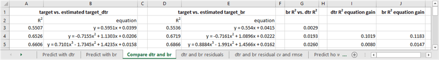
The following table from an Excel worksheet may highlight more clearly differences between the two model types and the functions for relating estimated target values to observed target values. By the way, observed and estimated target values were copied and pasted from SQL Server to Excel. There was no need to do any programming or even create an SSIS solution. After the transfer of data from SQL Server to Excel, the analyses were implemented within Excel.

• Columns A and B from the Excel worksheet below shows the R² value and equation for fitting estimated target values from a decision tree model to observed target values with three different functions – linear, quadratic, and cubic.
• Columns D and E shows the same kind of outcomes for a bagged regression model.
• As noticed in the discussion of the preceding graphical comparisons, the R² value was always greater for the bagged regression model (examine column G for confirmation of this). No matter what function was used to relate estimated target values to observed target values, the bagged regression model always returned a superior fit. Furthermore, the degree of superiority grew as the functions changed successively from a linear function to a quadratic function and ultimately to a cubic function.
• As the functions for relating the estimated target values to observed target values progressed from linear to quadratic to cubic, the fit improved.
  • This trend is confirmed independently for a decision tree regression model and a bagged regression model.
  • Column I confirms this trend for a decision tree model, and Column J confirms this trend for a bagged regression model.

Computing model variance and model bias based on a bagged regression training set sample

Model variance and model bias are two widely used techniques for comparing models. Model variance can be operationalized as the ratio of the standard deviation for the estimated target values divided by the average of the estimated target values. This ratio is often referred to as the coefficient of variation. The smaller the coefficient of variation for a model, the less variability there is for the estimates from a model. Provided the model is relatively accurate, a smaller coefficient of variation for a model is better than a larger coefficient of variation.

Bias for an individual data point reflects how accurate the estimated target value is relative to the observed target value. Across all the data points to which a model is fit. The root mean squared error (rmse) is often used to assess the bias of a model.

One common way to assess the bias of a data point is to compute the difference of the observed target value less the estimated target value for the data point. This is often called a residual. You can compute model bias as the square root of the average of the squared residuals; this quantity is typically referred to as the root mean squared error (rmse). When comparing models to assess bias, you can compare the rmse for two different models over the same set of data points. The model with the rmse that is closest to zero has the least model bias.

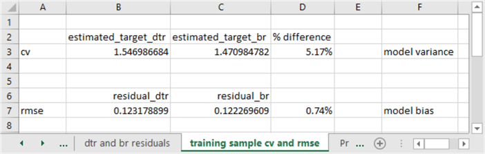
The following screen shot shows the model variance and model bias for the decision tree regression model versus the bagged regression model.

• The coefficient of variation for the decision tree regression model is 5.17 percent greater than for the bagged regression model. In other words, the bagged regression model estimates have a smaller model variance than the decision tree regression model. The bagged regression model wins because it is better to have a smaller model variance.
• The rmse for the bagged regression model is .74 percent different than the decision tree regression. This percent difference is exceedingly small; the difference is essentially immaterial. An R² analysis of the bagged regression squared residuals versus the decision tree regression squared residuals results in a value of nearly 1. This confirms that the predictions from both models have approximately equal bias. The models tie on model bias. The model bias is exceedingly small overall and the bias is about the same between the two models.

Results from comparing models with the hold-out sample

This section performs the same analyses as in the previous section however, the analyses are for a different group of dataset rows. Because the dataset rows are different, the observed and estimated target values are also different. It is common in data science modeling projects to evaluate model performance with more than one group of observed and estimated target values. When an outcome appears consistently over two or more groups of observed and estimated target values, this consistency confirms the use of the model outcome for making predictions about other groups of observed and estimated target values.

The sample of observations in the previous section consisted of 400 weather observations used for training the bagged regression model. Recall that the sample in the previous section was randomly drawn with replacement from an original population of the 294 distinct weather observations. The "with replacement" condition means that some weather observations can occur more than once among the 400 rows of weather observations. In fact, there are just 221 unique weather observation row values among the set of 400 weather observation row values.

This section analyzes observed and estimated target values for the 73 observations not selected for training the bagged regression model. The sub-section titled "Data for comparing models based on the hold-out sample" shows representative values from this hold-out sample.

Calculating regression estimated values with the hold-out sample

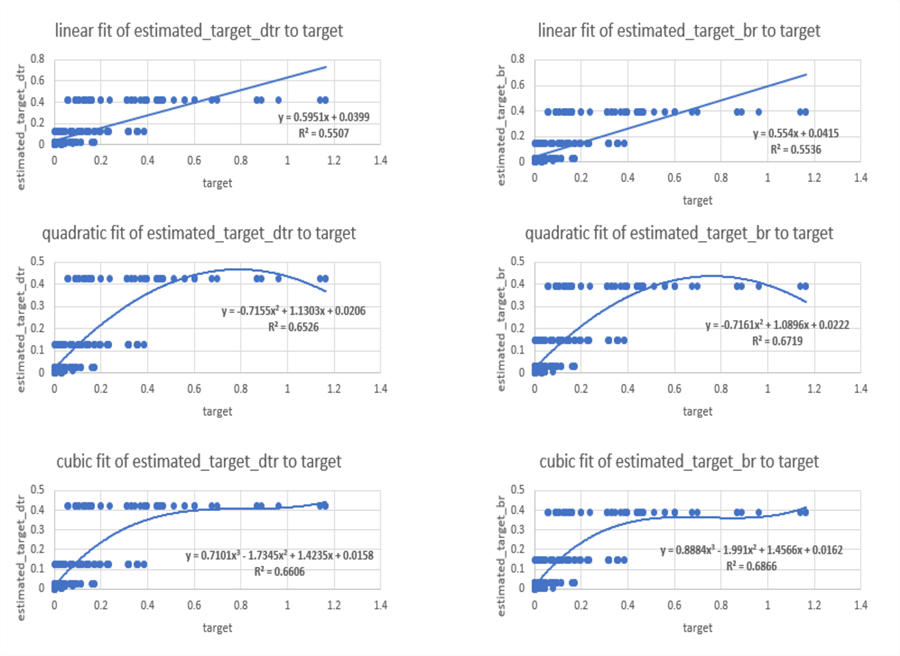
The following set of images compares the estimated target observations versus the observed target values over the 73 hold-out weather observations.

• The left column uses the decision tree model to compute estimated target values and the right column uses the bagged regression model to compute estimated target values.
• The images in the left and right columns use three different functions for the smooth lines through the data points.
  • The top pair of charts shows a linear function through the estimated and observed target values.
  • The middle pair of images shows a quadratic function through the estimated and observed target values.
  • The bottom pair of charts shows a cubic function through the estimated and observed target values.

If you carefully examine the charts it will become apparent that the quadratic and cubic functions do a better job of accounting for estimated values with observed values than the linear function. The superiority of the quadratic and cubic functions is most obvious for larger observed target values. The cubic function fits the estimated and observed values more closely than the quadratic function.

The following table from an Excel worksheet highlights numerically key points in the preceding charts.

• Columns A and B show the R² values and equations for each of the three functions for the smoothed lines through the estimated and observed target values where estimated values come from the decision tree regression model.
• Columns D and E show the R² values and equations for each of the three functions for the smoothed lines through the estimated and observed target values where estimated values come from the bagged regression model.
• Column G shows the R² values for the function based on the bagged regression model estimated target values less the R² values for the function based on the decision tree regression model estimated target values.
• Columns I and J show the R² gains for higher order polynomial functions versus lower order polynomial functions or polynomial functions versus linear functions through the estimated target values. Column I is for the decision tree regression model results and Column J is for the bagged regression model results.
  • Cell I4 shows the R² gain of the quadratic function over the linear function for the decision tree regression model.
  • Cell I5 shows the R² gain of the cubic function over the quadratic function for the decision tree regression model.
  • Cell J4 shows the R² gain of the quadratic function over the linear function for the bagged regression model.
  • Cell J5 shows the R² gain of the cubic function over the quadratic function for the bagged regression model.

Unlike the bagged regression training set, the hold-out sample does not show a consistent pattern of higher R² values for functions through the estimated target values from the bagged regression model than the decision tree regression model.

Nevertheless, there is a consistent tendency across both the bagged regression training set and the hold-out samples for higher-order polynomials to have a higher R² value than a lower-order polynomial or a linear function. Furthermore, the magnitude of the advantage is greater for the bagged regression model than for the decision tree regression model.

Computing model variance and model bias based on a hold-out sample

This sub-section shows the percentage difference in terms of model variance and model bias between the two model types. The results in this sub-section are for the hold-out sample. The comparable results for the other sample used in this tip appears in the "Computing model variance and model bias based on a bagged regression training set sample" sub-section.

The model variance is smaller for the bagged regression model than the decision tree regression model with the hold-out sample as well as the bagged regression training set sample. It is advantageous to have a smaller model variance. It is commonly reported that bagged regression models have smaller model variance than decision tree regression models (here and here). This tip also supports this common finding. The model variance advantage for a bagged regression model follows from the fact that the average standard deviation across a set of bagged samples is smaller than in a whole sample without bagging. Such as is used to compute estimated target values with decision tree regression.

Assessing model bias between two models depends on the absolute value of the size of the difference between each of the models. Within this tip, the size of the difference between models is close to zero for both samples (absolute value of .74 percent with the bagged regression training set sample and absolute value of 1.19 percent with the hold-out sample). Furthermore, an R² analysis of the bagged regression squared residuals versus the decision tree regression squared residuals results in a value of nearly 1 which indicates that the estimates from both models have approximately equal bias. This outcome is because both models have the same structure.

In conclusion, both models have small bias and the square residuals from both models map each other nearly perfectly. However, the bagged regression model is better than the decision tree regression model. This is because the smaller model variance of a bagged regression model keeps its estimated target values closer to observed target values.

Next Steps

This tip's download includes four files:

• a .sql file that extracts from a SQL Server weather data warehouse the data used in this tip
• a PowerPoint file with the two decision tree diagrams displayed in the "An overview of the decision tree and bagged regression models" section
• an Excel workbook file containing the expressions used to compute values for the comparison of the decision tree model and bagged regression model
• an Excel workbook file with a tab for each of the sample datasets evaluated in this tip

After you confirm the sample works for the code, worksheet analyses, and data in the download for this tip, you can implement the same general approach to data within your organization.

Many web pages around the internet describe how to create a decision tree regression and bagged regression models as well as how to compare them.

• Here is a basic presentation on decision tree regression models: Decision Tree - Regression
• Here is a basic presentation of bagging: Bagging, and here is a more advanced presentation on bagging which is available from this seminal source: Bagging Predictors
• Here are several presentations on comparing bagged regression to decision tree regression: Bagging and Random Forest Ensemble Algorithms for Machine Learning, Boosting, Bagging, and Stacking — Ensemble Methods with sklearn and mlens, and Bagging Vs Boosting In Machine Learning

About the author

Rick Dobson is an author and an individual trader. He is also a SQL Server professional with decades of T-SQL experience that includes authoring books, running a national seminar practice, working for businesses on finance and healthcare development projects, and serving as a regular contributor to MSSQLTips.com. He has been growing his Python skills for more than the past half decade -- especially for data visualization and ETL tasks with JSON and CSV files. His most recent professional passions include financial time series data and analyses, AI models, and statistics. He believes the proper application of these skills can help traders and investors to make more profitable decisions.

This author pledges the content of this article is based on professional experience and not AI generated.

View all my tips