Problem
I found a prior tip that used SQL Server to compare leveraged and unleveraged ETFs as long-term investments. I presented the example to my investing club. My fellow club members recently asked how to use SQL Server to mine inverse ETFs to uncover hints about how to trade them on a short-term basis. Please present some T-SQL code samples, results sets, and charts illustrating how to mine inverse ETFs to evaluate trading strategies.
Solution
Mining projects start with a collection of data for the mining project. One especially robust and relatively easy way to collect historical price and volume data for an ETF ticker is to use the Yahoo Finance manual interface for downloading historical data to the download folder of your computer. Yahoo Finance does not charge for using this interface or the data it provides. A prior MSSQLTips.com tip (Migrating Time Series Data to SQL Server from Yahoo Finance and Stooq.com) walks you through how to use the interface in its "Using the Yahoo Finance user interface" section.
This tip focuses on inverse ETFs. For readers unfamiliar with inverse ETFs, this tip starts with a short section describing them. You may also find a prior tip (SQL Server Data Mining for Leveraged Versus Unleveraged ETFs as a Long-Term Investment) on comparing leveraged and unleveraged ETFs, which has helpful information about ETFs for you. The prior tip additionally includes sample T-SQL code for transferring historical ticker price and volume data downloaded from Yahoo Finance to a SQL Server table.
After populating a SQL Server table with some data, you need to explore the table. This exploring is what we mean by mining. Charts are an especially useful tool in the early stages of a mining project. SQL Server is great at storing data and can also be used for more precise mining via queries. However, SQL Server does not generate charts via T-SQL code. Therefore, this tip copies the collected data from the SQL Server to Excel to create line charts. If you prefer to use another charting package besides Excel, you may find it convenient to export CSV files from SQL Server to Python. Python interfaces with multiple graphing libraries. Two prior tips illustrating the use of these graphing libraries are Plotting in Python for Financial Time Series Data for Exponential Moving Averages and How to Visualize Timeseries Data with the Plotly Python Library.
What are Leveraged Inverse ETFs?
An ETF is a security like a company’s stock, except that prices on successive trading days are for a collection of stocks or an index instead of just one individual company. This feature allows an investor to gain the benefits of diversity by investing in just one financial security.
A leveraged ETF has a leveraging factor for translating daily percent price changes for an ETF relative to its underlying basket of securities or index:
- If the basket changes its price from the open through the close of a trading day by 2% and the leveraging factor is 3, then the ETF price increases by 6% from the open through the close of the trading day.
- If the basket changes its price by -2% during a trading day and the leveraging factor is 3, then the ETF price declines by 6% from the open through the close of the trading day.
Inverse ETFs exist as pairs of ETFs with positive and negative leveraging factors relative to the same underlying index. One member in an ETF pair has a positive leveraging factor, and the other member in an inverse pair has a negative leveraging factor. These inverse pairs are meant for relatively short-term trades.
- By owning an inverse ETF with a negative leveraging factor, the worth of your equity increases as the ETF price declines.
- By holding an inverse ETF with a positive leveraging factor, the worth of your equity increases as the ETF price increases.
- Because ETF prices do not always either increase or decrease, these securities are meant for relatively short-term trades.
- When an ETF price is increasing, owning an ETF with a positive leverage factor can be profitable.
- When an ETF price is decreasing, owning an ETF with a negative leverage factor can be profitable.
- The challenge with this type of security is to know when to buy and sell ETFs with a positive or negative leverage factor.
This tip examines the price behavior of two pairs of ETFs (BOIL vs. KOLD and TQQQ vs. SQQQ). The tip additionally includes in its download file two more pairs of ETFs (JNUG vs. JDST and SOXL vs. SOXS) for you to mine on your own. The following table shows the tickers for all eight ETFs as well as their leveraging factor and the name of the underlying index.
| Table for Inverse Leveraged ETFs | ||
|---|---|---|
| Ticker | Leverage Factor | Name of Underlying Index |
| BOIL | 2 times | Bloomberg Natural Gas Subindex |
| KOLD | -2 times | Bloomberg Natural Gas Subindex |
| JNUG | 3 times | S&P/TSX Venture Composite Index |
| JDST | -3 times | S&P/TSX Venture Composite Index |
| SOXL | 3 times | PHLX Semiconductor Index |
| SOXS | -3 times | PHLX Semiconductor Index |
| TQQQ | 3 times | Nasdaq-100 Index |
| SQQQ | -3 times | Nasdaq-100 Index |
Getting to Know This Tip’s Data
The data for this tip resides in the symbol_date table of the dbo schema within the DataScience database. The download file for this tip includes CSV files from Yahoo Finance for each of the eight ticker symbols in the preceding table. You can change the source database according to your computing environment.
Here is a script to display all the rows in the symbol_date table. The rows are sorted by Symbol and Date column values because of a primary key for these columns in the symbol_date table.
select [Symbol]
      ,[Date]
      ,[Open]
      ,[High]
      ,[Low]
      ,[Close]
      ,[Volume]
from [DataScience].[dbo].[symbol_date]
Here are a pair of excerpts showing the first and last three rows from the results set returned by the preceding script.
- The first row is for the first date, 2020-01-02. The last row is for the last date data was collected in this tip (2023-10-30).
- The first symbol in alphabetical order is BOIL. The last symbol in alphabetical order is TQQQ. Recall that there are tickers in the download file for this tip.


Here is a script to display three aggregate values for each symbol in the tip’s source data.
- The aggregate values are the start date (min(date)), end date (max(date)), and number of trading days (count(*)) for each symbol.
- A subquery in the script restricts the results set to one row per symbol. The group by clause at the end of the script orders the rows by symbol.
-- start and end dates for ETF tickers
-- along with count of trading days per ETF ticker
select
 symbol
,min(date) [start date]
,max(date) [end date]
,count(*) [number or trading days]
from  [DataScience].[dbo].[symbol_date]
where symbol in
(
select distinct symbol
from  [DataScience].[dbo].[symbol_date]
)
group by symbol
Here is a screenshot with the results set from the preceding script. This sample of trading data has a start date of 2020-01-02 and an end date of 2023-10-30 for each ticker symbol. There are 964 trading days in this date range for each ticker symbol.

A Closer Look at This Tip’s Data
The following script populates the #temp table based on a select statement with a derived table in its from clause. The from clause joins the BOIL close column values and the KOLD close column values on matching date values from the symbol_date table in the dbo schema of the DataScience database. The main body of the select statement uses case statements to populate the Boil_is_greater and Kold_is_greater_or_equal columns with category values of:
- ‘BOIL is greater’ or Null.
- ‘KOLD is greater or equal’ or Null.
The two new columns identify each row in #temp as one in which either:
- b_close is greater than k_close (‘BOIL is greater’).
- k_close is greater than or equal to b_close (‘KOLD is greater or equal’).
The select statement at the end of the script displays all the rows in the #temp table.
Use DataScience
go

drop table if exists #temp

-- to designate rows as
-- BOIL is greater or KOLD is greater or equal
-- in #temp
select
 *
,
case
 when b_close > k_close then 'BOIL is greater'
 else Null
end Boil_is_greater
,
case
 when k_close >=b_close then 'KOLD is greater or equal'
 else Null
end Kold_is_greater_or_equal
into #temp
from
(
-- join of BOIL and KOLD closes by date values
select b.Date, b.[Close] b_close, k.[Close] k_close
from
(
(select date,[close] from dbo.symbol_date where symbol = 'BOIL') b
join
(select date,[close] from dbo.symbol_date where symbol = 'KOLD') k
on b.Date = k.Date
)
) assign_Bold_is_greater_or_Kold_is_greater_or_equal

select * from #temp
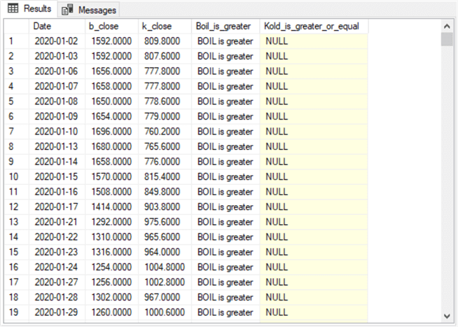
The following sequence of screenshots shows results set excerpts and matching images of selected rows from the #temp table. Rows are denoted by row number in the sequence of screenshots.
The immediately following screenshot shows the first 19 rows in the #temp table. All 19 Bold_is_greater column values contain ‘BOIL is greater’. This is because the b_close column value for each row is greater than the corresponding k_close column value.
The next screenshot excerpts 19 subsequent rows with row numbers 50 through 68 from the #temp table:
- Rows 50 and 51 are for the final two non-null ‘BOIL is greater’ rows from the sequence of rows starting in row 1 of the preceding screenshot.
- Rows 52 through 66 all have ‘KOLD is greater or equal’ in their Kold_is_greater_or_equal column.
- Row 67 has a value of ‘BOIL is greater’ in its Boil_is_greater column.
- Row 68 has a value of ‘KOLD is greater or equal’ in its Kold_is_greater_or_equal column.

The next screenshot displays a line chart from Excel based on rows 52 through 66 in the preceding screenshot. The orange line is for k_close values. The blue line is for b_close values. The orange line is always above the blue line, which indicates that all k_close values are greater than b_close values from 2020-03-17 through 2020-04-06.

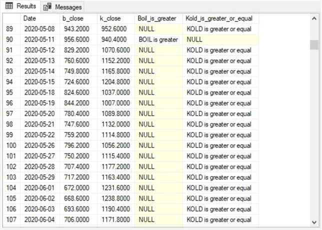
The next pair of screenshots contain excerpts for rows 91 through 148 for the results set in the #temp table. This is a second block of rows with trading dates from 2020-05-12 through 2020-08-03. All column values have ‘KOLD is greater or equal’ in their Kold_greater_or_equal column.
Here is a line chart from Excel based on rows 91 through 148. This is the second line chart for this tip. Notice that the orange line for k-close values is consistently above the blue line for b_close values.

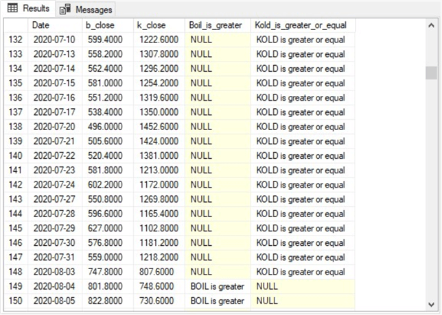
The next block of rows is for a third line chart that contains data from row 91 through row 179 in the following screenshot.
- This block of rows has one set of rows in which the k_close values are all greater than the b_close values. This block of rows begins in row 91 and extends through row 148.
- The second block of rows for the third line chart starts with rows 149 and 150 from the screenshot just before the second line chart. Additionally, the rows in the third line chart continue through row 179, which appears in the following results set excerpt. All the rows in this second block of rows contain ‘BOIL is greater’ in the BOIL_Is_greater column.

Here is the line chart for the content in rows 91 through 179. Notice that this range includes one block of rows where the orange line values are above the blue line values, followed by another block of rows where the blue line values are above the orange line values. The range of rows matching the blue line is for rows where ‘BOIL is greater’ in the BOIL_Is_greater column.

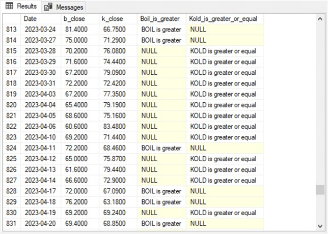
The following pair of screenshots is for data in 2023. The range of rows for the following line chart begins with row 815 in the first results set excerpt and runs through row 872 in the second results set excerpt. The first and last set of rows from SQL Server are followed by a line chart of the data from Excel. The fourth line chart for this set of rows shows a pattern of changing orientations between the orange and blue lines. Furthermore, the line orientations change rapidly. When this kind of pattern manifests itself in time series data, you may find it useful to exclude the data from your analysis.


A Mining Data Analysis
The main reason for the mining demonstration in this tip is to equip you to specify and evaluate rules for determining when to buy and sell profitably leveraged inverse ETFs. The preceding section shows that leveraged inverse ETFs sometimes have alternating blocks of dates when one ETF rises from below to above its corresponding inverse ETF. This section examines whether it is possible to devise and evaluate decision rules for buying and selling inverse ETFs based on the total set of rows for the BOIL and KOLD inverse ETFs as well as a second set of inverse ETFs – namely for the TQQQ and SQQQ ETFs.
The prior section shows that alternate rising and falling of inverse ETF close prices happen sometimes, but not always. It is well known that there is a high degree of randomness to security prices over time. One approach to preparing time series for analysis is to filter out dates with irregular sequential price data. This section shows the impact of manually filtering categorized time series data, like the values examined in the preceding section.
In particular, the filter searches for four consecutive trading days with this pattern
- The first two consecutive trading days must belong to the last two days of a block of trading days during which one member of a pair of inverse ETFs, such as KOLD, is below its corresponding ETF, such as BOIL.
- The third consecutive trading day must be the first trading day of a new block of at least two or more trading days where the order of the close prices for the tickers flip. For example, if the close price of the KOLD ticker rose from below to above the close price for the BOIL ticker on the third day, then this criterion is satisfied (and one or more shares of KOLD are purchased).
- The fourth consecutive trading day is a test day. No matter what, the decision rule sells shares for the ETF at the close price on the fourth trading day. For example,
- If the KOLD ticker close price of the fourth day rises above the close ticker price on the third day, then the decision rule wins.
- If the KOLD ticker close price on the fourth day does not rise above the KOLD ticker price on the third day, then the decision rule loses.
- The amount of the gain or loss depends on the difference in the close prices for KOLD on third and fourth trading days, respectively.
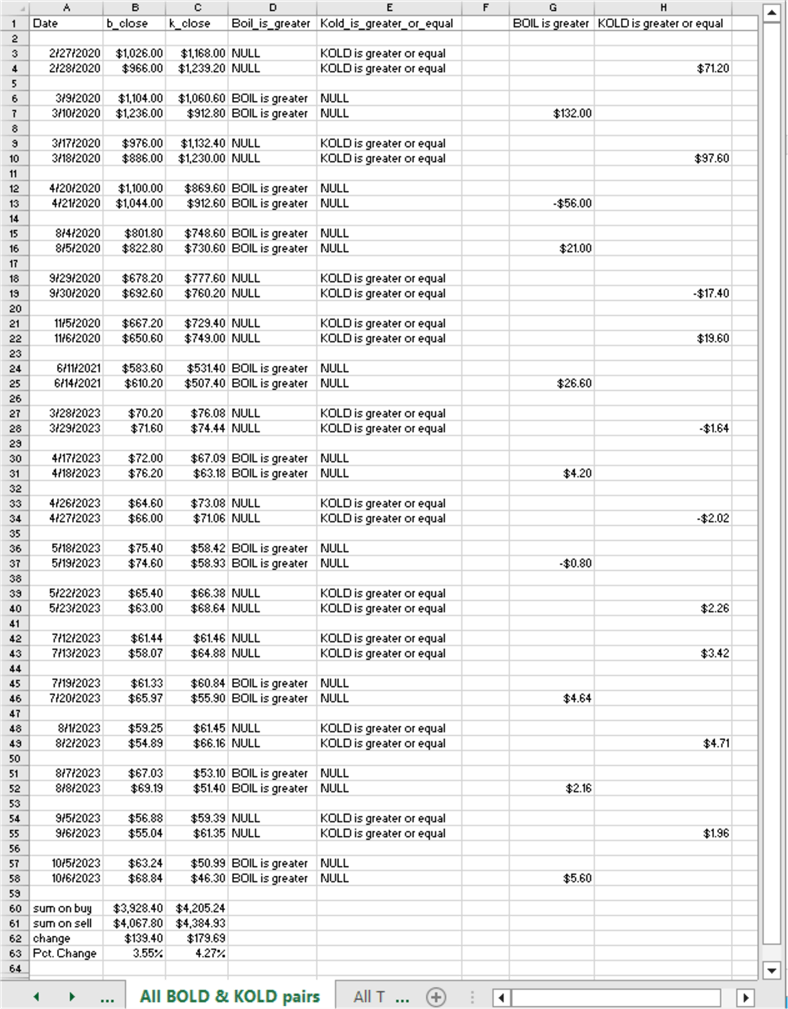
The filtered trade results are displayed and summarized for the KOLD and BOIL tickers in the following screenshot.
- The Date column values (from column A) denote the third and fourth consecutive trading dates for successive buy and sell dates.
- The values in columns G and H show the difference in close prices between successive trading dates.
- Column G shows the difference in BOIL close prices on the third and fourth trading days when the BOIL close price transitions from a value below KOLD to a value above KOLD on the third consecutive trading date.
- Column H shows the difference in the close prices on the third and fourth trading days when the KOLD close price transitions to a value from below BOIL to a value at or above BOIL on the third consecutive trading date.
- There are 19 pairs of trading dates summarized in the following screenshot.
- Cells A60 through C63 summarize the results across the 19 trading day pairs.
- The average percentage change in close prices is 3.55% for b_close values.
- The average percentage change in close prices is 4.27% for k_close values.
The filtered trade results are displayed and summarized for the TQQQ and SQQQ tickers in the following screenshot.
- The Date column values (from column A) denote the third and fourth consecutive trading dates for successive filtered trades.
- The values in columns G and H show the difference in close prices between successive trading dates.
- Column G shows the difference in TQQQ close prices on the third and fourth trading days when the TQQQ close price transitions to a value from below SQQQ to a value above SQQQ on the third consecutive trading date.
- Column H shows the difference in the close prices on the third and fourth trading days when the SQQQ close price transitions to a value from below TQQQ to a value at or above TQQQ on the third consecutive trading date.
- There are seven pairs of trading dates summarized in the following screenshot.
- Cells A24 through C27 summarize the results across the seven trading day pairs.
- The average percentage change in close prices is 1.74% for t_close values.
- The average percentage change in close prices is 1.42% for s_close values.

This is my first attempt at a decision rule and an analysis of results for leveraged inverse ETF pairs. The results are impressive for a first attempt. This is because the decision rule yielded successful outcomes for both pairs of leveraged inverse ETFs on more than half the filtered consecutive four-day test periods. It is possible that alternative decision rules may yield even more successful outcomes.
Next Steps
If you wish to grow your skills for projects like the one in this tip, you may start with the sample data and T-SQL code in the download file for this tip. The file has two types of contents.
- The first type contains price and volume data in CSV files for each of the eight ticker symbols (KOLD, BOIL, SQQQ, TQQQ, JDST, JNUG, SOXL, and SOXS). Four of these ticker symbols were examined in this tip. Four additional ticker symbols are available for you to replicate and extend the analysis steps in this tip with fresh data.
- The second type contains the T-SQL script that I used to migrate the CSV files to a SQL Server table ([DataScience].[dbo].[symbol_date]). You can add a primary key constraint based on symbol and date column values to the symbol_date table so that select statements return rows in time series order within symbols without needing an order by clause.
The decision rule for evaluating the historical price data is applied via manual inspection of the rows in the #temp table. This tip describes the decision rule criteria in “A Mining Data Analysis” section.
After successfully loading the data and manually implementing the decision rule, you can try the next steps.
- Programmatically implement the decision rule with T-SQL for the #temp table. In the past, I have found T-SQL lag functions are useful for this kind of task.
- Devise and implement alternate decision rules that are evaluated programmatically. Your goal will be to find one or more decision rules that perform more successfully than the decision rule analyzed in this tip.

Rick Dobson is a SQL Server professional with decades of T-SQL experience that includes authoring books, running a national seminar practice, working for businesses on finance and healthcare development projects, and serving as a regular contributor to MSSQLTips.com. He has been a practicing Python developer for more than the past half decade – with a special emphasis for data visualization and ETL tasks with JSON and CSV files. His most recent professional passions include financial time series data and analyses, AI models, and statistics. If you are interested in growing your skills in any of these areas especially as they relate to financial securities, consider visiting his blog at https://securitytradinganalytics.blogspot.com/2023/12/.
- MSSQLTips Awards: Leadership (200+ tips) – 2025 | Author of the Year Contender – 2017-2024