How to Comparatively Assess Buy-Sell Models with SQL Server

By: Rick Dobson   |   Updated: 2022-09-23   |   Comments   |   Related: > TSQL

Problem

I am a SQL professional seeking to grow my skills in investment analytics. Please present a framework for comparing buy-sell models based on tables saved in SQL Server. I am particularly interested in comparing the model tables via the compound annual growth rate metric.

Solution

A buy-sell model can accept open and close prices for a financial security over successive trading days from a start date through an end date as input. The model searches for a succession of buy dates, each followed by a matching sell date. The objective of the model is to discover buy-sell date pairs with higher sell prices than matching buy prices.

The buy dates and sell dates from a buy-sell model often depend on one or more price indicators, such as MACD indicators, RSI indicators, moving average crossover indicators, candlestick patterns, or Heikin Ashi candlestick values, as well as model rules for specifying when to buy and sell a security based on the indicators. The indicators and model rules can signal buy and sell actions. The buy and sell prices can depend on open prices (or some derivative of an open price like the price 30 minutes after the open).

By assessing the accumulated account balances from a succession of buy-sell cycles from a start date through an end date, you can determine which set of price indicators and model rules are better at growing an initial account balance. The compound annual growth rate (CAGR) is a metric that assesses the rate of accumulated wealth from a set of model rules for specifying buy and sell dates. This tip shows how to accept a table of buy and sell prices and compute with SQL code the CAGR. While there is more to assessing a model than comparing the rate of accumulated wealth, this metric is often of central interest when comparing buy-sell models.

This tip is a walkthrough for comparatively assessing two different buy-sell models with the CAGR metric.

Overview of Transforming Trading Date and Price Tables to Buy-Sell Cycle Tables

The following illustration displays top-line elements for building a buy-sell model. The model-building process starts with a table of open, high, low, and close prices along with volume data for successive trading dates. This initial table can contain more data than is used for comparative model assessments. For example, the source data is likely to have data for more symbols and more dates than are used in any specific set of model assessments.

Therefore, the original source data is commonly filtered to create a table with the data for a model run. There are likely to be at least two main filtering steps. First, you must filter the original source data for the ticker belonging to a particular security. Second, you can filter the data for a specific timeframe, such as for the trading dates in 2021, 2020, and 2019.

After filtering the original source data table into a table for a model run, you can apply the code for the buy-sell model to the filtered data. The model's output from the SQL code will be a table of buy-sell cycles. Each row in the buy-sell cycle table can have an identifier as well as buy and sell prices for each buy-sell cycle (along with whatever other data items the model reports).

The following screenshots display the buy-sell table from the model described in this prior tip. The model aims to discover profitable trades for the AAPL ticker for Apple, Inc. The trading dates for this example are for the years 2021, 2020, and 2019.

• The first screenshot displays the first 40 rows of the buy-sell table.
  • Trade number column values denote successive buy-sell cycles.
  • The buy_price and sell_price columns indicate the buy and sell price for each successive trade.
  • The rate of return column is the sell_price column value less the buy_price column value divided by the buy_price column value for up to four places after the decimal point.
    • If the rate of return is positive, then that is a winning trade that increases the balance in a trading account from a preceding period.
    • If the rate of return is not positive, then that is not a winning trade, and the account balance during that trade declines or remains the same.
  • The winning trade column is 1 when the sell_price column value is greater than the buy_price column value.
  • The cumulative balance amt column shows how an initial balance of $1000.00 changes over successive trades.
    • The cumulative balance amt column value rises on a winning trade row.
    • The cumulative balance amt column value declines on a losing trade row.
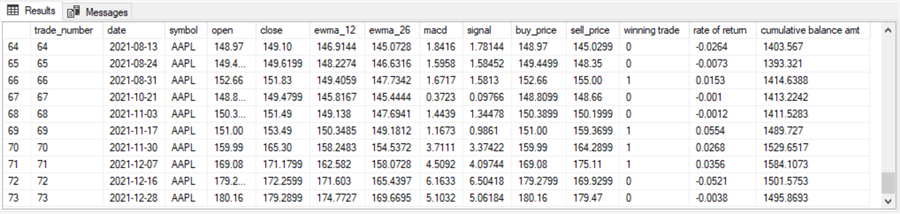
• The second screenshot shows the cumulative balance amt column values for the remaining 33 trades in the set of buy-sell cycles for this model.
  • As you can see, the 73^rd trade has a final "cumulative balance amt" of $1495.8693. This represents a total gain of nearly 50 percent over the initial balance of $1000.
  • After reporting the "cumulative balance amt" for the final trade, the code returns the CAGR across the three years from 2021 back through 2019. The compound annual growth rate (CAGR) is 14.36 percent. A subsequent section will describe the computational process and provide more commentary on interpreting CAGR values, but it may help to motivate you to read the rest of this tip that a CAGR of 14.36 is a pretty good result.

Code Example for Computing a Buy-Sell Cycle Table

The two models compared in this tip use a subset of the MACD indicators with different model rules for designating buy and sell dates. The first model is presented and described in this prior tip. The second model is the focus of this other tip - How to Build a Data Science Time Series Model with SQL.

Here is a slightly modified version of the code to pull the open and close prices for the AAPL ticker symbol. The original version of this script appears in the tip for the first model.

• The script below pulls data from the yahoo_finance_ohlcv_values_with_symbol SQL Server table. The data was collected from Yahoo Finance and deposited into a table in SQL Server.
• The SELECT statement in the script extracts four columns ([date], [symbol], [open], and [close]) from the yahoo_finance_ohlcv_values_with_symbol table and inserts them into the #temp_for_ewma temp table.
• The select statement also designates three other columns
  • ewma_12 and ewma_26 column values are updated elsewhere in the model code to compute MACD indicators
  • row_number column values are populated by the SQL Server row_number () function. Financial time series processing often benefits from row_number () function values because stock markets close on weekend days and selected holidays. Therefore, you cannot reference dates to obtain sequential time series values. However, the row_number column values provide an index series for sequential time series values.
• The @symbol local variable is assigned the string value ‘AAPL' for Apple, Inc. A comment on the same line as the @symbol assignment shows tickers for the full set of six tickers tracked in this tip. A WHERE clause within the script specifies the collection of rows from the yahoo_finance_ohlcv_values_with_symbol table for the current value of @symbol.

use DataScience
go
 
-- use this segment of the script to set up for calculating
-- ewma_12 and ewma_26 for ticker symbol
 
-- initially populate #temp_for_ewma for ewma calculations
-- @ewma_first is the seed
-- time series data are from dbo.stooq_prices for @symbol symbol
declare @symbol varchar(5) = 'AAPL' --'AAPL', 'GOOGL', 'MSFT', 'SPXL','TQQQ', 'UDOW'
declare @ewma_first money = 
(select top 1 [close] from dbo.yahoo_finance_ohlcv_values_with_symbol where symbol = @symbol order by [date])
 
-- create and populate base table for ewma calculations (#temp_for_ewma)
 
drop table if exists #temp_for_ewma
 
-- ewma seed run
select 
 [date]
,[symbol]
,[open]
,[close]
,row_number() OVER (ORDER BY [Date]) [row_number]
,@ewma_first ewma_12
,@ewma_first ewma_26
into #temp_for_ewma
from dbo.yahoo_finance_ohlcv_values_with_symbol
where symbol = @symbol
and [date] >= 'January 1, 2011'
order by row_number
 
-- optionally echo #temp_for_ewma before updates in while loop
   select * from #temp_for_ewma order by row_number

Here are screenshots of the first and last ten rows from the preceding script to initialize the #temp_for_ewma table.

• The first date in the table is for January 3, 2011. This is because January 1 and January 2 in 2011 are weekend days.
• Also, notice that January 8 and January 9 in 2011 are missing; these two dates are also weekend dates.
• The open and close column values are for open and close prices on a trading date.
• The row_number column values start with a value of 1 and increase by 1 for each sequential time series row in the source data. These rows exclude weekend dates and stock market holidays, such as Thanksgiving Day and Labor Day.
• The ewma_12 and ewma_26 column values will eventually be populated with exponentially weighted close column values. These values are computed and assigned to the columns later in the model code. At this point in the script, the same value is assigned to all rows in the ewma_12 and ewma_26 columns.
• The last date in the second screenshot is for February 18, 2022, and the other rows in the second screenshot are also for the year 2022. A WHERE clause, such as those appearing in the next script excerpt, can filter out all these dates from 2022 if your goal was to process data from trading dates in 2019, 2020, and 2021.

Additional code in the full model script filters the rows from the original source data into one of three different timeframes. The following excerpt from a subsequent select statement shows the code for selecting dates in one of three timeframes.

• The first WHERE clause can pull data from 2021, 2020, and 2019.
• The second WHERE clause can pull data from 2018, 2017, and 2016.
• The third WHERE clause can pull data from 2015, 2014, and 2013.

Expose only one of the three WHERE clauses without a comment marker depending on the timeframe for which you want to process data. The example below processes data for trading dates in 2019, 2020, and 2021.

from #temp_for_ewma
where year(date) in (2021,2020,2019)
--where year(date) in (2018,2017,2016)
--where year(date) in (2015,2014,2013)

Accumulating Account Balance Amounts after Successive Buy-Sell Cycles with a Model

This tip reports on the change in account balances for two different models developed with a gap of about six months. The model rules for picking buy and sell dates are different for each model.

Cumulative Account Balances for the First Model

The next code segment accumulates balance amounts over successive buy-sell cycles. This code segment depends on the existence of a #buy_price_sell_price table. This table was generated with SQL code, available in the download for this tip. The results are for the first buy-sell model. The table's first and last ten rows appear in the following two screenshots.

• The trade_number column has a separate value for each buy-sell cycle.
• The buy_price and sell_price columns contain buy and sell prices for each buy-sell cycle. These values are determined by the underlying data and the model rules for designating buy and sell dates.
• The buy_price and sell_price column values can be used to determine
  • If a buy-sell cycle is a winning trade
  • The rate of return during the buy-sell cycle, and
  • The cumulative account balance through the end of the current buy-sell cycle starting from a specified initial balance. In this tip, the initial balance is set to $1000.
• The last three column values are null in the following screenshots.

Here is the code for populating the last three columns in the #buy_price_sell_price table with non-null values.

• As you can see, the code depends on a loop that passes through successive buy-sell cycles. The process is iterative because the cumulative balance for each row in the #buy_price_sell_price table is dependent on the cumulative balance from the prior row (or the initial balance in the case of the first row) and the rate of return in the current row. In this tip, the initial balance is assigned a value of $1000.
• The code inside the while loop updates the three null column values for the current row, and it then sets up for the next row by:
• Updating the pointer for the current row (@current_trade_number) to point at the next buy-sell cycle
  • Assigning the current row's "cumulative balance amt" column value to the @balance_amt local variable, this local variable makes the prior row's "cumulative balance amt" column value available when computing the cumulative balance amt column value for the next row.

-- loop sequentially through trades
-- to assess if @current_trade_number is a winner ([winning trade])
-- the rate of return for the current trade, and the
-- cumulative balance through the current trade
-- save the computed results in the #buy_price_sell_price table
 
declare
   @balance_amt money = 1000,
   @number_of_trades int =
      (select count(*) from #buy_price_sell_price),
   @current_trade_number int = 1,
   @rate_of_return real
 
 
while @current_trade_number <= @number_of_trades
begin
 
   -- update [winning trade], [rate of return], and [cumulative balance amt]
   -- for @current_trade_number
   update #buy_price_sell_price
      set [winning trade] =
            case
               when sell_price > buy_price then 1
               else 0
            end,
         [rate of return] = ((sell_price - buy_price)/buy_price),
         [cumulative balance amt] =
            case
               when trade_number = 1 then ( 1 + ((sell_price - buy_price)/buy_price)) * @balance_amt
               else ( 1 + ((sell_price - buy_price)/buy_price)) * @balance_amt
            end
   where trade_number = @current_trade_number;
 
   -- set @balance_amt to [cumulative balance amt] from @current_trade_number
   set @balance_amt
      = (
         select [cumulative balance amt]
         from #buy_price_sell_price
         where trade_number = @current_trade_number
        )
 
   -- increment @current_trade_number by 1
   set @current_trade_number = @current_trade_number +1
 
end
 
-- optionally echo #buy_price_sell_price table results set
   select * from #buy_price_sell_price

Here are the first and last ten rows from the #buy_price_sell_price table after the preceding code segment runs.

• Notice how the "cumulative balance amt" column value increases when the winning trade column has a value of 1. The amount of the increase is dependent on the rate of return value.
• In contrast, the "cumulative balance amt" column value for the current row will be less than (or, at the most, equal to) the cumulative balance through the prior row. In the case of a non-winning trade, there is a decrease in the "cumulative balance amt" column nearly all the time.

Cumulative Account Balances for the Second Model

The code for the second model assessed in this tip also generates a buy-sell cycle table based on its model rules about when to buy and sell a security. Instead of characterizing each buy-sell cycle by its rate of return during a cycle, the code for the second model tracks the change in the number of shares held during a cycle.

• At the beginning of the first buy-sell cycle, the model computes the number of security shares held as $1000 divided by the cost per share of a security, which is the buy price. The number of shares is calculated to the full precision of a float value – not just up to four places after the decimal, as is the case for the rate of return in the first model.
• At the end of the first buy-sell cycle:
  • The model recalculates the account balance as the product of shares of a security held times the cost per share of a security at the end of the first buy-sell cycle, which is the sell price
  • This product of the two multiplied values is the cumulative account balance at the end of the first cycle
• At the beginning of the next buy-sell:
  • The model recalculates the shares of a security held at the beginning of the current buy-sell cycle as cumulative account balance at the end of the preceding buy-sell cycle divided by the buy price for the current buy-sell cycle
  • At the end of the current buy-sell cycle, the cumulative account balance for the current buy-sell cycle is recalculated as the product of the shares of a security held times the sell price at the end of the current buy-sell cycle
• The two steps in the preceding bullet are repeated for as many remaining buy-sell cycles as in the set of buy-sell cycles for the model data.

Here is a script from the second model for creating the buy-sell cycle table, excluding the cumulative balances. The script consists of an outer query with two subqueries for derived tables.

• The into clause in the outer select statement populates a table named #for_second_macd_trade_model_with_buy_sell_prices. This table contains a row for each buy-sell cycle and six columns for each row. The columns are:
  • symbol for the ticker being processed
  • buy_sell_cycle_# for the buy-sell cycle identifier
  • buy_date and sell_date are, respectively, for the buy and sell dates of the current buy-sell cycle
  • buy_price and sell_price are, respectively, for the buy and sell prices of the current buy-sell cycle
• The first subquery has the name from_buy_rows, and the second subquery has the name from_sell_rows.
  • The source table for both subqueries has the name #for_second_macd_trade_model_with_sell_action. Although the table name ends with "sell_action," the source table contains information for both the buy action and the sell action in a buy-sell cycle.
    • The subquery for buy action events has a where clause of "where buy_action = 1". More importantly, this subquery returns values for the buy_date and buy_price columns.
    • The subquery for sell action events has a where clause of "where sell_action = 1". This subquery returns values for the sell_date and sell_price columns.
  • An inner join matches the rows from each subquery on the buy_sell_cycle_# column for the results set from each subquery
• A closing select statement in the following script displays the results sets from both subqueries in the #for_second_macd_trade_model_with_buy_sell_prices table.

-- extract buy_price and sell_price
-- for computing account balances
drop table if exists #for_second_macd_trade_model_with_buy_sell_prices
select
 from_buy_rows.symbol
,from_buy_rows.buy_sell_cycle_#
,buy_date
,sell_date
,buy_price
,sell_price
 into #for_second_macd_trade_model_with_buy_sell_prices
from
(
select
 symbol
,date buy_date
,[open] buy_price
,row_number() over (order by date) buy_sell_cycle_#
from #for_second_macd_trade_model_with_sell_action
where buy_action = 1
) from_buy_rows
 
join
 
(
select
 symbol
,date sell_date
,[open] sell_price
,buy_action
,row_number() over (order by date) buy_sell_cycle_#
from #for_second_macd_trade_model_with_sell_action 
where sell_action = 1
) from_sell_rows
on from_buy_rows.buy_sell_cycle_# = from_sell_rows.buy_sell_cycle_#
 
-- optionally echo #for_second_macd_trade_model_with_sell_action
  select * from #for_second_macd_trade_model_with_buy_sell_prices

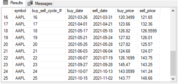
Here are the first and last ten rows from the #for_second_macd_trade_model_with_buy_sell_prices table. Notice there are just 25 cycles in the buy-sell table from the second model. In contrast, there are 73 cycles in the buy-sell table from the first model. This is because the first and second models have different rules for designating buy and sell actions.

Computing the Compound Annual Growth Rate with SQL

CAGR is a widely used metric for comparing investment strategies, hedge funds, or different types of investments. This metric smooths the rate of return across a timeframe, such as a range of years. The metric assumes any yearly gains or losses are folded into the cumulative account balance for the timeframe over which the CAGR is computed. This process results in a compound annual growth rate from the beginning through the end of a timeframe.

The expression for computing the CAGR depends on three terms:

• The initial deposit to an account before any changes in the first year of a timeframe
• The ending account balance in the final year of a timeframe
• The number for the years in a timeframe; if there are three full years in a timeframe, then the number is 3; if there are three and a half years in a timeframe, then the number is 3.5

The CAGR reveals the average annual rate across the years in a timeframe. It does not predict future results. It does not show the rate of change for individual years within a timeframe. When comparing two or more models, the CAGR model can conclusively show which model had the highest average annual rate of return across a timeframe.

In the context of the current tip, three timeframes are used:

• From the beginning of 2013 through the end of 2015; this timeframe is designated as t3
• From the beginning of 2016 through the end of 2018; this timeframe is designated as t2
• From the beginning of 2019 through the end of 2021; this timeframe is designated as t1

Because there are three years in each timeframe, the number of years per timeframe in each CAGR computation is 3.

The beginning balance for each symbol for each timeframe is $1000.00. The ending balance for each of the three timeframes is the cumulative balance after the last trade in a timeframe.

SQL Code for CAGR from the First Model

The following script is for computing the CAGR in the code from within the first model. The DECLARE statement for local variables at the top of the script excerpt references the beginning and ending balances with @initial_beginning_balance and @final_ending_balance local variables. The @symbol local variable value is computed as the distinct symbol column value in the #buy_price_sell_price table from within the first model; the code for populating this table appears in the preceding section. The number of years within a timeframe is always three years for this tip. Therefore, this term does not require a local variable.

After the DECLARE statement, two set statements in the script assign values to the @initial_beginning_balance and @final_ending_balance local variables. In this script example, a constant value of 1000 is assigned to the @initial_beginning_balance local variable. A SELECT statement extracts the cumulative balance amt column value from the last row in the #buy_price_sell_price table.

The main role of the last select statement in the script segment below is to compute the CAGR value based on the @initial_beginning_balance and @final_ending_balance local variable values and the three years in a timeframe. The @symbol value in the select statement identifies for which ticker symbol the computed CAGR belongs.

-- parameters for identifying @symbol and computing CAGR
 declare
  @initial_beginning_balance money,
  @final_ending_balance money,
  @symbol nvarchar(10) =  (select distinct symbol from #buy_price_sell_price)
 
-- compute @initial_beginning_balance and
-- @final_ending_balance for CAGR expression
 
set @initial_beginning_balance = 1000
 
 
set @final_ending_balance =
  (select [cumulative balance amt]
   from #buy_price_sell_price
   where trade_number =
   (select max(trade_number) final_buy_sell_cycle
    from #buy_price_sell_price)
  )
 
-- 1.0 over 3 instead of 1 over 3 is required to avoid truncation
-- of exponent value in CAGR expression
 
select
  @symbol [symbol],
  round(
  (power((@final_ending_balance/@initial_beginning_balance),(1.0/3))-1)
  *100  ,2) CAGR

The following screenshot shows the CAGR value computed by the preceding script. It indicates that the initial balance of $1000 grows at a rate of 14.36 percent for each of the three years in the timeframe. Recall that this is nearly a 50 percent increase across the three years in timeframe t1.

If you grow $1000 by 14.36 percent, and then grow that value by 14.36 percent, and then grow that value by 14.36 percent, the final ending balance is $1495.624. However, the ending balance is $1495.8693 to four places after the decimal as computed within the "Cumulative account balances for the first model" subsection. One critical issue for this difference is the floating-point approximation for the exponent (1.0/3) in the CAGR expression. There is no precise value in a binary number system for (1.0/3) from base 10; this is also true for many other rational numbers. Therefore, the floating-point processor within a computer chooses the closest value it can within a binary number system to represent the result.

SQL Code for CAGR from the Second Model

The code in the "Cumulative account balances for the second model" subsection shows how to compute the #for_second_macd_trade_model_with_buy_sell_prices table in the second model. This table includes a results set for the second model with the buy date and sell date for each buy-sell cycle as well as the buy and sell price for each buy-sell cycle. Given this table, the script in this section can compute the beginning balance and the ending balance for each buy-sell cycle.

Here is the code for computing the beginning and ending balances from the #for_second_macd_trade_model_with_buy_sell_prices table in the second model.

• The script segment starts with a DECLARE statement for a set of local variables to facilitate the computation of beginning and ending balances for each buy-sell cycle. The DELCARE statement specifies the name and data type for each local variable, and it also initializes selected other local variables.
• Next, the code creates a fresh copy of the #buy_sell_cycle_balances table. This table contains six columns with values for each buy-sell cycle in the second model:
  • current_buy_sell_cycle is an identifier for each successive buy-sell cycle
  • beginning_balance is the balance before the start of the current buy-sell cycle
  • buy_price is the buy price for the current buy-sell cycle
  • sell_price is the sell price for the current buy-sell cycle
  • buy_volume is the number of shares held for the current buy-sell cycle
  • ending_balance is the balance after the end of the current buy-sell cycle
• A while loop after the CREATE TALBE statement for the #buy_sell_cycle_balances table populates successive rows in the table and manages a local variable (@current_buy_sell_cycle) for navigating between consecutive rows in the table.
• After the while loop passes through all rows in the #buy_sell_cycle_balances table, a select statement optionally prints the populated version of the table.

-- declare local variables for populating #buy_sell_cycle_balances table
declare @buy_sell_cycles int = (select max(buy_sell_cycle_#) from #for_second_macd_trade_model_with_buy_sell_prices),
    @current_buy_sell_cycle int = 1,
    @beginning_balance money = 1000.0000,
    @buy_price money,
    @sell_price money,
    @buy_volume float,
    @ending_balance money,
    @initial_beginning_balance money,
    @final_ending_balance money
 
-- #buy_sell_cycle_balances table to be populated in while loop
drop table if exists #buy_sell_cycle_balances
 
create table #buy_sell_cycle_balances(
current_buy_sell_cycle int,
beginning_balance money,
buy_price money,
sell_price money,
buy_volume float,
ending_balance money
)
 
-- loop to compute cumulative buy_sell_cycle balances
while @current_buy_sell_cycle <= @buy_sell_cycles
begin
 
select @buy_price = buy_price
  from #for_second_macd_trade_model_with_buy_sell_prices
  where buy_sell_cycle_# = @current_buy_sell_cycle
 
select @sell_price = sell_price
  from #for_second_macd_trade_model_with_buy_sell_prices
  where buy_sell_cycle_# = @current_buy_sell_cycle
 
-- must cast @buy_price as float to get buy_volume to correct fractional value
select @buy_volume = (@beginning_balance)/cast((@buy_price) as float)
 
select @ending_balance = @sell_price*@buy_volume
 
insert into #buy_sell_cycle_balances
select @current_buy_sell_cycle [@current_buy_sell_cycle],
      @beginning_balance [@beginning_balance],
      @buy_price [@buy_price],
      @sell_price [@sell_price],
      @buy_volume [@buy_volume],
      @ending_balance [@ending_balance]
 
-- point at next buy sell cycle
-- and set @beginning_balance for next buy sell cycle
set @current_buy_sell_cycle = @current_buy_sell_cycle + 1
set @beginning_balance = @ending_balance
 
end
 
-- optionally echo #for_second_macd_trade_model_with_sell_action
   select * from #buy_sell_cycle_balances

Here are screenshots of the first and last ten rows in the table for the AAPL ticker symbol.

• The first column contains buy-sell cycle identifier numbers.
• The second and sixth columns contain, respectively, beginning and ending balances for each buy-sell cycle.
• The buy_price and sell_price column values are extracted from the underlying #for_second_macd_trade_model_with_buy_sell_prices table.
• The buy_volume column is the number of shares of a security held for a buy-sell cycle.
• The beginning _balance is the account balance just before the start of a buy-sell cycle.
  • The initial beginning _balance column value is defined as $1000.
  • Subsequent beginning_balance column values are assigned the ending_balance of the previous buy-sell cycle.
• The buy_volume column value is computed as the beginning_balance column divided by the buy_price column value.
• The ending_balance column value is the buy_volume column value times the sell_price column value.
• The last select statement optionally displays all the row values for the six columns in the #buy_sell_cycle_balances table. These values are derived as described in the preceding steps.

The second model's code for computing the CAGR for a symbol, such as AAPL, for a timeframe, such as the one with data from 2021 through 2019, appears below. This code cannot run on its own; it must run in the same scope as the preceding script.

-- compute @initial_beginning_balance and
-- @final_ending_balance for CAGR expression
 
set @initial_beginning_balance =
  (select beginning_balanc
   from #buy_sell_cycle_balances 
   where current_buy_sell_cycle = 1
  )
 
set @final_ending_balance =
  (select ending_balance
   from #buy_sell_cycle_balances
   where current_buy_sell_cycle =
   (select max(current_buy_sell_cycle) final_buy_sell_cycle
    from #buy_sell_cycle_balances)
  )
 
-- populate @symbol
declare @symbol nvarchar(10) =
  (select distinct symbol
   from #for_second_macd_trade_model_with_buy_sell_prices)
 
 
-- 1.0 instead of 1 over 3 is required to avoid truncation of exponent value
 
select
  @symbol [symbol],
  round(
  (power((@final_ending_balance/@initial_beginning_balance),(1.0/3))-1)
  *100  ,2) CAGR

Here is the output from the preceding script segment. It shows the CAGR for the AAPL ticker from the second model for the timeframe with data from 2019 through 2021.

In this comparison of the CAGR values, model 1 generated a more profitable outcome (14.36) than the outcome for model 2 (9.19).

Summary of Model Outcomes for the First and Second Models

This tip shows how to compare via the CAGR two models that specify when to buy and sell securities. Both models specify buy dates when the MACD line rises above its signal line. Conversely, both models specify sell dates when the MACD line crosses below its signal line. A primary difference between the models is that the first model does not start to specify buy dates until after the MACD line crosses above its centerline value. At the same time, the second model does not specify buy dates unless the MACD line is below its centerline value. See the tips for the first model and the second model (How to Build a Data Science Time Series Model with SQL) for additional details about each model.

The code for each model is available in this tip's download. The code for each model was run eighteen times – once for each combination of ticker symbol and timeframe date range. The six ticker symbols are AAPL, GOOGL, MSFT, SPXL, TQQQ, and UDOW. The timeframe ranges are for trading dates in 2021 through 2019, 2018 through 2016, and 2015 through 2013. As a result, there are 18 CAGR values for the first model and 18 corresponding CAGR values for the second model. The following table shows:

• The CAGR values for each model for timeframe-symbol combinations.
• The difference between each pair of CAGR values.
• The average CAGR values for each model as well as the difference between the models.

Notice that the average CAGR values for the first and second models are around 12 percent – 11.81 percent for the first model and 12.55 for the second model.

How do you know what a good CAGR is? The internet search for this tip discovered a range of values and opinions to answer the question. The opinions indicate that the answer can depend on the size of the companies in a portfolio, the reason you are investing (for example, a child's college tuition versus supplemental retirement income for social security), or even the tolerance of an application for price volatility.

In the internet search for this tip, around 7 to 10 percent rates were considered adequate. Rates of greater than 10 percent and into the mid-teens were considered good for a quality portfolio of securities that was well managed. Rates above the mid-teens were for those who sought extraordinary gains and could tolerate a higher probability of capital loss. Here are a few references for you to get started deciding what might be a "good" CAGR value for your application requirements:

• What Is Considered a Good Return on Investment?
• What is a Good Return on Investment?
• What is a Good CAGR Percentage?

Based on these guidelines, the 12 percent CAGR for both models in this tip is a "good" return. However, please be aware that in any one timeframe for one security, the rates can vary widely from the average CAGR across a range of securities in different timeframes.

Now that you know the average CAGR for each of the two models covered in this tip is "good," we can ask whether there is a significant difference between the models. The answer from the table above is no. On average, you can achieve about the same "good" return with either of the two models. However, the models are also clearly different in how they achieve their "good" returns. The first model can require dramatically more buys and sells to get to the same return as the second model – at least, this was the case for the AAPL ticker in the 2021 through 2019 timeframe.

Next Steps

• The download for this tip contains two T-SQL scripts – one for the first model and the other for the second model. The editions of the scripts in the download let you run the whole script from beginning to end for the combination of a single ticker and a timeframe. The scripts from the download display the CAGR for a combination of symbol and timeframe values. The script for the first model requires you to update the timeframe twice for each run of the model, but the second model only requires one timeframe update for a single run of the model. You can also edit the script for each model to display selected intermediate values as described and illustrated in the text and screenshots within this tip.
• In addition to the scripts, this tip's download includes CSV files with the raw time series data for each of the six tickers referenced. Load the CSV files into the yahoo_finance_ohlcv_values_with_symbol table referenced if you care to run the code as described in this tip.
• The last download element is an Excel spreadsheet with the summary results for the 18 combinations of symbols and timeframe values for each model.

About the author

Rick Dobson is an author and an individual trader. He is also a SQL Server professional with decades of T-SQL experience that includes authoring books, running a national seminar practice, working for businesses on finance and healthcare development projects, and serving as a regular contributor to MSSQLTips.com. He has been growing his Python skills for more than the past half decade -- especially for data visualization and ETL tasks with JSON and CSV files. His most recent professional passions include financial time series data and analyses, AI models, and statistics. He believes the proper application of these skills can help traders and investors to make more profitable decisions.

This author pledges the content of this article is based on professional experience and not AI generated.

View all my tips