Building a SQL Computational Framework for MACD Indicators

By: Rick Dobson   |   Updated: 2022-12-15   |   Comments   |   Related: > TSQL

Problem

I belong to a data engineering team at a financial consulting firm. A growing number of our clients use MACD indicators in custom trading strategies. Our firm uses SQL Server to store underlying prices for MACD indicators as well as for computing MACD indicator values. We seek an example of a general computational framework for MACD indicators to better serve our clients.

Solution

MACD indicators were originally formulated and promoted by Gerald Appel in the late 1970s. These technical indicators continue to attract widespread attention from technical analysts, traders, and academic scholars. The Next Steps section of this tip includes a starter set of references for readers who want to grow their understanding of MACD indicators.

The objective of the framework is to present techniques for programming MACD indicators in SQL Server. Three prior tips illustrate applications in SQL Server for MACD indicators (buy/sell signals for securities, mining price time series data, and building data science models for time series data), but these prior tips do not examine the details of how to compute MACD indicators.

While this tip highlights SQL programming guidelines for computing MACD indicators, it is common to encounter SQL programming requirements that include the need to perform a set of interrelated calculations. If your SQL programming must compute any kind of values, then this tip may provide helpful design guidelines. You may also find value in how the framework from this tip adapts stored procedures to compute a basic kind of calculation, such as an exponential moving average. This tip even includes a use case example for applying the same stored procedure to different source datasets without using dynamic SQL.

A Brief Overview of MACD Indicators

The MACD indicators examine from different perspectives changes between two different exponential moving averages of a security's price over a set of time periods. The two types of averages are for a fast and a slow exponential moving average. A fast average has a relatively short period length so that it follows underlying securities prices more closely than a slow average with a longer period length.

When computing exponential moving averages for MACD indicators, the fast average has a default period length of 12, and the slow average has a default period length of 26. Some technical analysts use different period lengths for different types of securities, such as stocks, crypto currencies, or gold, or different period durations, such as hours, days, or weeks.

Exponential moving averages require at least two prices in a time series. The second and all subsequent prices in a time series can serve as a basis for computing an exponential moving average value. Furthermore, you can compute a fast and a slow average for each price in a time series after the first price.

Here is the general expression for an exponential moving average (ema) of a time series of prices for a security. Notice that the ema at time t depends on two terms the price at time t and the ema at time t-1. Therefore, the exponential moving average for the initial period (t-1) is null because this period has no prior ema. This tip (and other sources for computing ema values) assigns the price from the initial period (t-1) as the ema for time t:

ema(t) = (alpha* price(t)) + ((1-alpha)*ema(t-1)

• price(t) is the security price at time t
• ema(t-1) is the exponential moving average at time t-1
• alpha and (1-alpha) are smoothing values for sequential moving averages

The smoothing values of alpha and (1-alpha) sum to 1. For financial applications, alpha typically depends on the following expression:

(2/(period_length+1))

Therefore, for MACD applications with the default settings, the fast ema has an alpha value of:

(2/(12+1))

In contrast, the slow ema with the default settings has an alpha value of:

(2/(26+1))

As you can see, both the fast and slow ema expressions put a larger weight on the most recent price relative to the prices in the ema preceding the most recent period. Also, the fast ema expression puts a relatively larger weight on the most recent price than the prices in the slow ema expression.

After computing the fast and slow ema values, you can start using the expressions for MACD indicators. These are three indicators:

• MACD line = fast ema – slow ema
• Signal line = ema with a default period length setting of 9 for the MACD line values
• Histogram = MACD line – Signal line

The Signal line indicator is an exponential moving average of the MACD line indicator. As with the fast ema and slow ema values, you can use other values than the default period length of 9.

Because the signal line is an exponential moving average that depends on the MACD line, which also depends on exponential moving averages, the signal line value is null for the first and second time periods. The Histogram value is computed as the scalar value difference of the MACD line value less the signal line value for a time period. The Histogram value is null for the first two rows because either or both of its terms are null in one of the first two periods.

Importing Time Series Prices

To compute MACD indicators in SQL Server, you must have access to historical price time series data for one or more tickers. This section demonstrates how to import previously downloaded data from another SQL Server application. For example, a prior tip, Correlating Stock Index Performance to Economic Indicators with SQL and Excel, downloaded historical prices for the SPY, QQQ, and DIA tickers. These three tickers are for exchange traded funds that track, respectively, the daily prices of the S&P 500, the NASDAQ 100, and the Dow Industrial Average indexes. The historical price and volume data collected in the prior tip are available in three csv files that are included in the download for this tip as well. The csv file names are:

• SPY_from_yahoo_on_10_31_2022.csv
• QQQ_from_yahoo_on_10_31_2022.csv
• DIA_from_yahoo_on_10_31_2022.csv

The following script shows the code for populating two different SQL Server tables with data from each of the files. The first table is named dbo.from_yahoo. This table is successively populated with each of the three csv files listed above. The csv files do not include a column for the ticker to which the historical price data belongs. The second table (dbo.symbol_date) is a copy of selected price and volume data from the first table as well as an additional column for the ticker. Therefore, the dbo_symbol_date table can hold data for all three tickers. The symbol column for the ticker value permits the retrieval of data for one ticker at a time.

As you can see, the script uses a bulk insert command to successively populate the dbo.from_yahoo table from each of the three csv files. After each cycle of populating a fresh version of the dbo.from_yahoo table, selected contents are transferred to the dbo.symbol_date table. Therefore, at the end of the script, the dbo.symbol_date table contains a separate set of rows for each ticker.

The total number of trading days for each ticker are different. This is because each of the tickers initially became listed on a stock exchange at a different date. While the starting date varies by ticker, the data for all three tickers in this tip conclude on October 31, 2022.

It may be worth pointing your attention to the fact that price values are saved in columns with a Decimal (19,4) data type instead of a money data type. These two data types often behave similarly. However, when you are dividing monetary values, the money and Decimal (19, 4) data types behave differently. The MACD indicators in this tip do not divide monetary values by other money values or a scalar value. However, it is possible for a quantitative analyst to specify computations that do involve the division of monetary values that will lead to different results between money and Decimal (19,4) data types. It turns out that the difference results from a truncation that causes the money data type to systematically underestimate the outcome for some divisions. Therefore, it is safer to use the Decimal (19,4) data type when working with monetary values. You can learn more about these data type differences in a prior tip titled "Money and Decimal Types for Monetary Values with SQL Server".

use DataScience
go
 
drop table if exists dbo.from_yahoo
 
create table dbo.from_yahoo(
   [Date] [date] NULL,
   [Open] DECIMAL(19,4) NULL,
   [High] DECIMAL(19,4) NULL,
   [Low] DECIMAL(19,4) NULL,
   [Close] DECIMAL(19,4) NULL,
   [ADJ Close] DECIMAL(19,4) NULL,
   [Volume] float NULL
)
go
 
drop table if exists dbo.symbol_date
 
create table dbo.symbol_date(
   [Symbol] nvarchar(10) not NULL,   
   [Date] [date] not NULL,
   [Open] DECIMAL(19,4) NULL,
   [High] DECIMAL(19,4) NULL,
   [Low] DECIMAL(19,4) NULL,
   [Close] DECIMAL(19,4) NULL,
   [Volume] float NULL
)
go
 
alter table symbol_date
add constraint pk_symbol_date primary key (symbol,date);
 
----------------------------------------------------------------------------------------------------------
 
-- bulk insert raw download for SPY into dbo.from_yahoo
bulk insert dbo.from_yahoo
from 'C:\DataScienceSamples\Correlating_index_etfs_with_econ_indicators\SPY_from_yahoo_on_10_31_2022.csv'
with
(
    firstrow = 2,
    fieldterminator = ',',  --CSV field delimiter
    rowterminator = '\n'
)
 
-- echo bulk insert
select * from dbo.from_yahoo
 
-- populate symbol_date with contents for SPY
insert into symbol_date
select
 'SPY' symbol
,cast([date] as date)
,[open]
,[high]
,[low]
,[close]
,[volume]
from dbo.from_yahoo
 
-- echo transferred data from dbo.from_yahoo
select * from symbol_date
 
----------------------------------------------------------------------------------------------------------
 
truncate table dbo.from_yahoo
 
-- bulk insert raw download for QQQ into dbo.from_yahoo
bulk insert dbo.from_yahoo
from 'C:\DataScienceSamples\Correlating_index_etfs_with_econ_indicators\QQQ_from_yahoo_on_10_31_2022.csv'
with
(
    firstrow = 2,
    fieldterminator = ',',  --CSV field delimiter
    rowterminator = '\n'
)
 
-- echo bulk insert
select * from dbo.from_yahoo
 
-- populate symbol_date with contents for SPY
insert into symbol_date
select
 'QQQ' symbol
,cast([date] as date)
,[open]
,[high]
,[low]
,[close]
,[volume]
from dbo.from_yahoo
 
-- echo transferred data from dbo.from_yahoo
select * from symbol_date
 
----------------------------------------------------------------------------------------------------------
 
truncate table dbo.from_yahoo
 
-- bulk insert raw download for QQQ into dbo.from_yahoo
bulk insert dbo.from_yahoo
from 'C:\DataScienceSamples\Correlating_index_etfs_with_econ_indicators\DIA_from_yahoo_on_10_31_2022.csv'
with
(
    firstrow = 2,
    fieldterminator = ',',  --CSV field delimiter
    rowterminator = '\n'
)
 
-- echo bulk insert
select * from dbo.from_yahoo
 
-- populate symbol_date with contents for SPY
insert into symbol_date
select
 'DIA' symbol
,cast([date] as date)
,[open]
,[high]
,[low]
,[close]
,[volume]
from dbo.from_yahoo
 
-- echo transferred data from dbo.symbol_date
select * from symbol_date

The next three screen shots show the first eight rows from both the from_yahoo and symbol_date tables for each of the three tickers. The top pane from each screen shot displays excerpted rows from the from_yahoo table, and the bottom pane from each screen shot displays excerpted rows from the symbol_date table. The first, second, and third screen shots are, respectively, for the SPY, QQQ, DIA tickers. Within this tip, the Close column values along with symbol and date column values are used to compute MACD indicators.

There is a different initial listing date for each of the three tickers. This date appears in the top row of each pane showing data in the from_yahoo table.

Computing Exponential Moving Averages for MACD Indicators

Exponential moving averages are computed three times on the way to computing MACD indicators: once for a column of fast ema values, a second time for a column of slow ema values, and a third time for a column of signal line values. Within this tip, the fast and slow ema column values are both computed from the Close column values with a SPY symbol value in the symbol_date table. The other two tickers (QQQ and DIA) in the symbol_date table are provided so that you can easily practice the use of the computational framework with the other tickers besides the one illustrated in this tip. The signal line ema values are based on the MACD line values, which are, in turn, dependent on columns of fast ema and slow ema values.

A single stored procedure named dbo.usp_ema_computer_with_dec_vals can compute all three sets of ema values. This tip's next section demonstrates how to run the stored procedure once for each set of ema values. The current section focuses on the code within the stored procedure. The stored procedure operates on a table named source_data. Before invoking the stored procedure, this table needs to be populated with appropriate column values if it does not already contain appropriate column values. Additionally, three parameter values need to be passed to the stored procedure when it is invoked. These parameters are:

• @symbol for the ticker value, which is SPY in the demonstration for this tip
• @period for the period length for the ema values. For the fast ema, slow ema, and signal line ema values with default settings, the @period parameter should be set, respectively, to 12, 26, and 9
• @alpha for one of the smoothing constants to be used when computing the fast or slow ema values or the signal line ema values. The computational framework relies on two smoothing constants based on the @alpha parameter
  • The @alpha smoothing constant is for the current period's price or MACD line value; @alpha's value is computed from this expression (2/(@period + 1))
  • The (1 - @alpha) smoothing constant is for the prior period's ema value

Here is the script to create the dbo.usp_ema_computer_with_dec_vals stored procedure. The script commences with a use statement to designate a default database name. Next, the code drops any prior version of the dbo.usp_ema_computer_with_dec_vals stored procedure in the default database. Then, a create procedure statement specifies the code for the stored procedure to run.

Within the create procedure statement, there are several main sections to implement the logic with SQL for computing an exponential moving average.

• The first section is comprised of three parameter declarations for @symbol, @period, and @alpha.
• Next, a begin…end block designates the computational code for the stored procedure.
  • This code starts by assigning the Close value from the first row in the source_data table to the @ema_first local variable
  • Next, the code creates a fresh copy of a temp table named #temp_for_ema. The temp table is created with the into clause in a select statement. The select designates the source_data table in the from clause for the select statement. All the rows in this initial version of the #temp_for_ema table have @ema_first as their ema column value. These column values are updated later in the script.
  • For example, an update statement assigns a null value to the ema column value in the first row of the #temp_for_ema table.
  • Next, a while loop with the help of three local variables processes successive pairs of rows from the third through the last row in the #temp_for_ema table.
    • On each pass a fresh ema value is computed by a set statement for the @today_ema local variable; this ema value is for the current row in the #temp_for_ema table
    • Then, the value of @today_ema is used to update the ema column value for the #temp_for_ema table
    • Next, the value of the @current_row_number local variable is increased by 1
    • When the value of @current_row_number is greater than @max_row_number, the while statement passes control to the next sql statement after the while loop
• A select statement after the while loop is the last statement in the stored procedure; it returns the fully updated #temp_for_ema table

use DataScience
go

-- create a fresh version of [dbo].[usp_ema_computer_with_dec_vals]
drop procedure if exists [dbo].[usp_ema_computer_with_dec_vals]
go

create procedure [dbo].[usp_ema_computer_with_dec_vals]
-- Add the parameters for the stored procedure here
@symbol nvarchar(10)  -- for example, assign as 'SPY'
,@period dec(19,4)     -- for example, assign as 12
,@alpha dec(19,4)      -- for example, assign as 2/(12 + 1)
as


begin
-- suppress row counts for output from usp
set nocount on;

-- parameters to the script are
-- @symbol identifier for set of time series values
-- @period number of periods for ema
-- @alpha weight for current row time series value

-- initially populate #temp_for_ema for ema calculations
-- @ema_first is the seed
declare @ema_first dec(19,4) = 
(select top 1 [close] from [dbo].[source_data] where symbol = @symbol order by [date])

-- create base table for ema calculations

drop table if exists #temp_for_ema

-- ema seed run to populate #temp_for_ema
-- all rows have first close price for ema
select 
[date]
,[symbol]
,[close]
,row_number() OVER (ORDER BY [Date]) [row_number]
,@ema_first ema
into #temp_for_ema
from [dbo].[source_data]
where symbol = @symbol
order by row_number

-- NULL ema values for first period
update #temp_for_ema
set
ema = NULL
where row_number = 1

-- calculate ema for all dates in time series
-- @alpha is the exponential weight for the ema
-- start calculations with the 3rd period value
-- seed is close from 1st period; it is used as ema for 2nd period

-- set @max_row_number int and initial @current_row_number
-- declare @today_ema
declare @max_row_number int = (select max(row_number) from #temp_for_ema)
declare @current_row_number int = 3
declare @today_ema dec(19,4)

-- loop for computing successive ema values
while @current_row_number <= @max_row_number
begin

set @today_ema =
(
-- compute ema for @current_row_number
select 
top 1
([close] * @alpha) + (lag(ema,1) over (order by [date]) * (1 - @alpha)) ema_today

from #temp_for_ema
where row_number >=  @current_row_number -1 and row_number <= @current_row_number
order by row_number desc
)

-- update current row in #temp_for_ema with @today_ema
-- and increment @current_row_number 
update #temp_for_ema
set 
 ema = @today_ema
where row_number = @current_row_number

set @current_row_number = @current_row_number + 1

end

-- display the results set with the calculated values
-- on a daily basis
select 
date
,symbol
,[close]
,@period period_length
,ema ema
from #temp_for_ema
where row_number < = @max_row_number
order by row_number

end
go

Computing the MACD Line Indicator from Fast and Slow ema Values

After you load the underlying data and create the usp_ema_computer_with_dec_vals stored procedure in the default database, you can start to implement the steps for computing the MACD line indicator. Recall that this indicator is the difference between two ema sets. One set is for fast ema values because it has a short period length that causes its ema values to quickly alter their values in response to the most recent underlying price changes. The other set is for a slower set of ema values with a longer period length that puts a relatively greater weight on prior ema values than the most recent price in the underlying data.

Here is a script for computing the MACD line indicator.

• It starts by designating a default database (DataScience).
• Next, it transfers data from the symbol_date table data to the source_data table in the dbo schema of the DataScience database. Also, a primary key constraint is added to the source_data table to help improve its performance in filters and joins with other tables.
• The next step is to create fresh versions of the fast_ema and slow_ema tables. These tables are named after the type of data they are designed to store.
• The next several lines of code run the stored procedure twice -- once with parameters for fast ema values and a second time with parameters for slow ema values.
  • Each exec statement for the stored proc is paired with an insert into statement for depositing the results set from the stored proc into the fast_ema or the slow_ema tables depending on stored procedure parameters
  • The code defining the contents of either results set is the select statement at the end of the preceding script
  • The code for each exec statement has the same overall structure, but each stored procedure call is different in a couple of ways
    • The first call readies data for the fast_ema table; it does this by specifying
      • An @period parameter value of 12 and
      • An @alpha parameter value of 0.1538, which is the quotient of 2 divided by 13 rounded to four places after the decimal point
    • The second call readies data for the slow_ema table; it does this by specifying
      • An @period parameter value of 26 and
      • An @alpha parameter value of 0. 0741, which is the quotient of 2 divided by 27 rounded to four places after the decimal point
    • Both stored procedure calls assign the same value (SPY) to the @symbol parameter
  • For demonstration purposes within this tip, this block of code ends with two select statements – one for the fast_ema table and the other for the slow_ema table
• The last block of code in the following script is for creating, populating, and displaying a fresh version of the temp table named #MACD.
  • The create table statement for the #MACD table designates three columns
    • the ticker symbol value (for an MACD line value)
    • the date (for an MACD line value)
    • the MACD line value
  • A select statement and its preceding insert into statement computes MACD line values and inserts them into the #MACD table
    • The specification for the third column in the #MACD table computes the MACD line value for a symbol and date as a fast ema value less a slow ema value
    • The from clause for the select statement is a derived table that performs an inner join between the fast_ema and slow_ema tables; the from clause also excludes rows with NULL MACD line values
  • Before displaying the contents of the #MACD table at the end of the script, the code adds a primary key constraint to the table to improve its performance and ensure that rows display in the order of the constraint key

use DataScience
go
 
-- populate dbo.source_data for [dbo].[usp_ema_computer_with_dec_vals] proc
-- based on dbo.symbol_date
drop table if exists dbo.source_data
 
select * into dbo.source_data from dbo.symbol_date
 
alter table source_data
add constraint pk_symbol_date_source_data primary key (symbol,date);
 
 
-- create fast_ema and slow_ema tables
drop table if exists fast_ema
go
 
create table dbo.fast_ema (
 date date
,symbol nvarchar(10)
,[close] dec(19,4)
,period_length dec(19,4)
,ema dec(19,4)
)
 
drop table if exists dbo.slow_ema
go
 
create table dbo.slow_ema (
 date date
,symbol nvarchar(10)
,[close] dec(19,4)
,period_length dec(19,4)
,ema dec(19,4)
)
 
 
-- compute fast_ema and slow_ema values for MACD line
-- @alpha parameter = 2/13 for @period = 12
-- @alpha parameter = 2/27 for @period = 26
-- compute @alpha rounded to 4 places after the decimal
insert into fast_ema
exec usp_ema_computer_with_dec_vals @symbol = 'SPY', @period = 12, @alpha = 0.1538
 
insert into slow_ema
exec usp_ema_computer_with_dec_vals @symbol = 'SPY', @period = 26, @alpha = 0.0741
 
-- echo fast_ema
select * from dbo.fast_ema
 
-- echo slow_ema
select * from dbo.slow_ema
 
 
-- compute MACD based on fast_ema - slow_ema
drop table  if exists #MACD
go
 
create table #MACD(
 symbol nvarchar(10) not null
,date date not null
,MACD dec(19,4) not null
)
 
insert into #MACD
-- remove initial MACD null column value
select 
 fast_ema.symbol
,fast_ema.date
,(fast_ema.ema - slow_ema.ema) MACD
from fast_ema inner join slow_ema on fast_ema.date = slow_ema.date
where (fast_ema.ema - slow_ema.ema) is not null
 
alter table #MACD
add constraint pk_symbol_date_#MACD primary key (symbol,date)
 
select * from #MACD

The following screenshot shows the first eight rows of the three results sets from the preceding script.

• The top pane is for a results set from the fast_ema table. Its period length is 12
• The middle pane is for a results set from the slow_ema table. Its period length is 26
• The bottom pane is for a results set from the #MACD table.
• Notice that the results set from the fast_ema and slow_ema tables have their initial date value on 1993-02-01 and their eighth entry on 1993-02-10. In contrast, the third results set for the #MACD table has an initial date of 1993-02-02 and its eighth entry on 1993-02-11.
  • Recall that the select statement for the #MACD table excludes rows with a null MACD column value. This exclusion is valid because there is no MACD value for 1993-02-01.
  • The NULL value for 1993-02-01 is because the expression for computing and exponential moving average requires at least one prior row, but the first row of underlying data on 1993-02-01 does not have a prior row.

Computing the Signal Line Indicator from the MACD Indicator

The signal line indicator values are just an exponential moving average of the MACD column values from the #MACD table. The default period length is 9 for computing signal line values as exponential moving average values from the MACD column values in the #MACD table. However, stock technical analysts sometimes use other period lengths besides the default value of 9. You can adapt the computational framework presented in this tip to other period lengths by updating the @period and @alpha parameters passed to the usp_ema_computer_with_dec_vals stored procedure. Recall that @alpha is based on period length. The expression for computing an @alpha parameter value based on a @period parameter value appears in the preceding script as well as in the "A brief overview of MACD indicators" section.

Here's the script for computing signal line values and joining them with MACD line values from the #MACD table and the close column values from the symbol_date table.

• After a use statement to reference a default database (DataScience), the script starts by creating and populating a fresh version of the source_data table that is derived from the #MACD table. Because the #MACD table is a local temporary table, it is convenient to have the script for creating the #MACD table connected to the Server and in the same sql file when the following script is run. This tip's download file includes the following script immediately after the preceding one on a single SSMS tab.
• Also, notice that the MACD column from the #MACD table receives an alias name of [close].
• The #MACD table with the freshly aliased column of MACD values is used to populate a fresh version of the source_data table. The source_data table also is assigned a primary key constraint based on its symbol and date column values.
• Next, a fresh version of the #Signal table is created. The column names for the #Signal table are date, symbol, MACD, period_length, and signal
• The #Signal table rows are populated with an insert into statement preceding an exec statement for the usp_ema_computer_with_dec_vals stored procedure. The parameters for the stored procedure in this example are
  • SPY for @symbol
  • 9 for @period
  • 0.2 for @alpha
• The rows in the #Signal table are echoed for you to familiarize yourself with the values returned by the stored proc
• The script concludes by left joining the #Signal table to the symbol_date table on both symbol and date column values. Recall that the symbol_date table is the SQL Server table with open, high, low, close, and volume data for all three tickers (SPY, QQQ, and DIA) in this tip's download file; the code, files, and sample data for the table are provided in the "Importing time series prices for this tip" section. A where clause in the select statement filters the symbol_date table for rows with a symbol column values of SPY; the symbol_date table in the example for this tip is populated with two other ticker values, which you can use for additional practice with the computing framework. Of course, you'll need to update the code slightly when working with data for other tickers besides SPY.
• Also notice that the where clause for the select query at the end of the script has a criterion to exclude rows with a null signal column value. It is convenient to use this filter because the usp_ema_computer_with_dec_vals stored procedure always returns a null exponential moving average value in its first row. Recall that this is because the expressions for computing an exponential moving average requires a prior column value for its underlying series, but this value is missing by definition from the first row.

use DataScience
go
 
-- compute signal as an exponential moving average
-- based on the MACD column values in the #MACD table
 
-- populate a fresh copy of dbo.source_data based on the #MACD table
-- for the usp_ema_computer_with_dec_vals proc
drop table if exists dbo.source_data
 
-- create and populate dbo.source_data from the #MACD table
-- designate an alias name [close] for the MACD column from the #MACD table
-- for use in the usp_ema_computer_with_dec_vals proc
select
 symbol
,date
,MACD [close]
into dbo.source_data
from #MACD
 
alter table source_data
add constraint pk_symbol_date_source_data primary key (symbol,date);
 
-- compute #Signal as an ema with a period length for the third MACD setting
-- default value is 9
 
drop table  if exists #Signal
go
 
create table #Signal (
 date date
,symbol nvarchar(10)
,[MACD]  dec(19,4)
,period_length dec(19,4)
,signal dec(19,4)
)
 
-- Compute signal column values as an exponential moving average
insert into #Signal
exec usp_ema_computer_with_dec_vals @symbol = 'SPY', @period = 9, @alpha = 0.2
 
-- display #Signal table rows with signal column values
-- computed from a 9 period length exponential moving average of MACD values
select * from #Signal order by date
 
-- left join #Signal to symbol_date to display
-- close, MACD, and signal values
select
 symbol_date.symbol
,symbol_date.date
,[close]
,#Signal.MACD
,#Signal.signal
from symbol_date
left join #Signal
on symbol_date.symbol = #Signal.symbol
and symbol_date.date = #Signal.date
where symbol_date.symbol = 'SPY'
 and #Signal.signal is not null

Here are some excerpts from the results sets in the preceding script:

• The top pane shows the first eight rows from the #Signal table, and the bottom pane shows the first eight rows from the #Signal table joined to symbol_date table
• Top pane data:
  • Starts with a date of 1993-02-02
  • Has a null signal column value on 1993-02-02, but other columns in the first row have non-null values
  • Has non-null signal column values for all rows after the first row
• Bottom pane data:
  • Starts with a date of 1993-02-03; notice that this is one trading date after the date for the top row in the top pane. This is because the select statement for the results in the bottom pane includes a criterion to exclude null signal column values
  • Has a column for close values; this column is missing from the top pane because the select statement for the top pane does not join the #Signal table with the symbol_date table (which is the source for the close column values)

Computing the Histogram Indicator from the MACD and Signal Indicators

The Histogram indicator is a much simpler indicator to compute than the MACD and signal indicators. The main reason for this is that you do not have to compute an exponential moving average to derive the Histogram indicator for a trading date. In fact, all you have to do is subtract the signal value from the MACD value for a trading date. When implementing data visualizations of Histogram values, it is common to display the values as a bar chart.

• If the MACD value is more positive than the signal value, then the bar extends upwards from the horizontal zero-line axis
• If the MACD value is less positive than the signal value, then the bar extends downwards from the horizontal zero-line axis

This tip section presents the numerical process for computing Histogram indicator values. A future tip will demonstrate ways to visualize MACD indicator values in line and bar charts. All you need to compute Histogram indicator values is a set of MACD and signal column values for trading dates. The bottom pane from the preceding figure shows that #Signal table can serve as a good source for computing Histogram indicator values. This is because the #Signal table has columns of both MACD and signal values.

The following script assumes you are running it in the same SQL Server session used to create and populate the #Signal table. One way to achieve this is to just run the code for this script immediately after the preceding script. The download for this tip provides a sample implementing this approach.

As you can see, the script contains a nested query that extracts data from both the symbol_date table and the #Signal table. The outer query displays all columns from the subquery and adds a new column based on MACD column values less signal column values from the subquery.

use DataScience
go
 
-- compute Histogram as MACD - signal
-- from for_Histogram
select
 for_Histogram.*
,(for_Histogram.MACD - for_Histogram.signal) Histogram
 from
 (
-- return #Signal table rows for the SPY ticker value
select
 symbol_date.symbol
,symbol_date.date
,[close]
,#Signal.MACD
,#Signal.signal
from symbol_date
left join #Signal
on symbol_date.symbol = #Signal.symbol
and symbol_date.date = #Signal.date
where symbol_date.symbol = 'SPY'
 ) for_Histogram

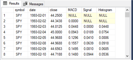
Here are the first eight rows from the results set from the preceding query.

• The Histogram values appear in the last column of the results set.
• The Histogram values for rows with dates of 1993-02-01 and 1993-02-02 are both null because one or both terms for the Histogram value are null.
• Histogram column values from 1993-02-03 on display with a decimal data type that specifies four places after the decimal point.

Next Steps

This tip's Solution section promised a selection of references for those who wanted to learn more about MACD indicators. Here is a short list of several references for your review. It is easy to find scores of references on the topic. If the references below do not satisfy your interest in the topic, an internet search will readily provide many more references for you to examine.

• The Complete Guide to MACD Indicator
• Ultimate Guide to MACD
• MACD (Moving Average Convergence/Divergence Oscillator)
• MACD

Some readers may also find value in prior MSSQLTips.com articles on MACD indicators (buy/sell signals for securities, mining price time series data, and building data science models for time series data).

The download files for this tip includes three SQL Server script files and three csv files.

• The first script file is named populate_symbol_date_in_DataScience.sql. This file draws on three csv files with open, high, low, close, date, and selected other data for the SPY, QQQ, DIA ticker symbols. You can use these four files to populate the original source data table from which excerpts show in the "Importing time series prices for this tip" section. You will need to run the first script file successfully to run the third script file.
• The second script file is named create_dbo_usp_ema_computer_with_dec_vals.sql. This script creates a stored procedure for computing exponential moving averages that can be customized by any of three parameters. You will need to run this script successfully in order to run the third script file.
• The third SQL Server script file named compute_slow_ema_fast_ema_MACD_Signal_Histogram.sql demonstrates how to compute MACD line values, signal line values, and Histogram values for the SPY ticker symbol. This file has three sections – one for each set of MACD indicators. Each set of indicators is stored in a temp table. Commentary in separate sections of this tip walks you through the code logic for each section.

A couple of interesting features are illustrated by the code samples:

• A stored procedure is demonstrated for computing an exponential moving average for a single ticker symbol. This stored procedure has considerable built-in flexibility because of three parameters for a ticker symbol, a period length, and a smoothing constant.
• The code also shows how to update an internal source data table for the stored procedure differently for MACD line values versus signal line values.
• The code in this tip is meant as a proof of concept – not a final solution for a production environment. The purpose of the code samples is to familiarize you with basic techniques for computing the three main types of MACD indicators for a single ticker symbol.
  • Your production requirement may not require all three MACD Indicators
  • or your requirements could easily involve the need to compute one or more MACD indicators for a large set of symbols.
  • Also, your requirements may benefit storing historical MACD indicator values and just updating previously computed indicator values as fresh data become available
• The code was unit tested repeatedly for the SPY ticker symbol, but no tests were performed for other tickers. Creative SQL programmers are likely to come up with code tweaks to enhance performance and/or flexibility. For example,
  • Omit select statements that merely echo results. This will make the code run faster at the expense of some transparency.
  • In many environments you may be able to achieve performance gains by using permanent SQL Server tables, instead of temp tables, for storing MACD indicator values.

About the author

Rick Dobson is an author and an individual trader. He is also a SQL Server professional with decades of T-SQL experience that includes authoring books, running a national seminar practice, working for businesses on finance and healthcare development projects, and serving as a regular contributor to MSSQLTips.com. He has been growing his Python skills for more than the past half decade -- especially for data visualization and ETL tasks with JSON and CSV files. His most recent professional passions include financial time series data and analyses, AI models, and statistics. He believes the proper application of these skills can help traders and investors to make more profitable decisions.

This author pledges the content of this article is based on professional experience and not AI generated.

View all my tips